Importing & Cleaning

Author

Christian McDonald

Goals of this lesson

In this second lesson we will work through building a notebook where you import data, manipulate it and do some analysis. While you may be viewing these lessons online, know they are also in the project folder all starting with lesson-. You’ll build your notebook in another file in practice-day1.qmd where you’ll be given some pre-written code with explanations of what it does. You’ll also write your own code with mini on-your-own quests.

In the end, we are creating a cleaned data set and exporting it to use later.

For this lesson we’ll be using daily weather summaries from Climate Data Online – daily temperature and precipitation readings.

Tip

Within a project I typically have one notebook for downloading and cleaning my data, and then another notebook for analyzing my data. Since this is a guided training, the organization of this project is a little different. We’ll walk through building a new project later.

Open the practice file

Let’s get started.

Make sure the Files page is open in the bottom right pane of RStudio.
Click on the gear icon and choose Go To Working Directory. This takes the file explorer to our project folder so we know where everything is.
Click and open the practice-day1.qmd file.

Our notebooks start with metadata at the top that includes the title listing, like this one, written in YAML and bracketed by the three dashes. There is other configuration you can do in the metadata, but we won’t here.

Below the metadata you’ll want to explain the goals of what you are doing in this notebook. We write these notes in Markdown in between our code.

Packages and libraries

After the goals in a notebook, the next thing to have is the libraries you’ll use. While there is a lot of functionality baked into R, users can also write and package pre-written code into libraries. Different libraries have different “functions” that we use to manipulate our data in some way. Learning how to use these functions IS programming.

We almost always load the tidyverse library which is actually a collection of libraries, including:

readr has functions that import and export data
dplyr has functions to manipulate data, like sorting and filtering
stringr helps us work with text
tidyr helps us shape data for different purposes
ggplot helps us visualize data through charts

We’ll use functions from all of these libraries, but they come in the one big toolbox, tidyverse.

We’ll use another function from another library, janitor to standardize some column names.

Here is how we set up the libraries. It is usually the first code chunk you’ll have in your notebook.

Tip

The code block below is displayed online in a special way to show you the tick marks, language designation and some execution options that are explained below. Usually the online directions only show the code inside the block.

This code chunk below has two special execution options that affect how the code works.

label: setup gives this chunk a special name that tells RStudio to run this block before any other if it hasn’t been run already.
message: false suppresses the usual messages we see in our notebook after loading libraries. With most code chunks we want to see these messages, but not this one because they are standard. Plus, I wanted to show you how the options work.

Execution options are not required, but those two are useful for our libraries chunk. That’s often the only place I use any.

```{r}
#| label: setup
#| message: false

library(tidyverse)
library(janitor)
```

In your practice notebook after the ## Libraries headline.
Use the copy icon at top-right to copy the contents of the code block listed above and paste it into your notebook.
Run the code block above using either the play button inside your Quarto document, or by placing your cursor in the code chunk and using Cmd-shift-return on your keyboard.

You’ll see a flash of green but you won’t see any feedback in your notebook because we suppressed it.

Functions

Those library() commands used above are what we call a function in R, and it is similar to formulas in a spreadsheet. They are the “verbs” of R where all the action happens.

Inside the parenthesis of the function we add arguments. In that library function it needed to know which package to load. Usually the first argument what data we are inserting into the function. There can be other options to control the function.

function(data, option_name = "value")

We can also string these functions together, taking the result of one and piping it into the next function. We’ll do that soon.

Importing data

We use functions from the readr library to import our data. We choose which function based on the format of the data we are trying to import.

The data I have prepared for you here is in “csv” format, or comma separated values. In this project we have two data folders, data-raw where we put our original data, and data-processed where we put anything we export out. Our aim here is to avoid changing our original raw data.

Important

From now on you’ll mostly create your own chunks in your practice notebook and type in the code indicated in the book. While it is possible to copy/paste the code easily, I implore you to type all the code here so you get used to using the RStudio editor.

After the ## Import headline and description there, insert a new code chunk. You can use the keyboard command Cmd+option+i or the green +C icon in the notebook toolbar.
Type in read_csv() into the code chunk. You’ll see type-assist trying to help you.
Once that is there, put your cursor in between the parenthesis (if it isn’t already) and type in an opening quote ". You’ll see that the closing quote is automatically added and your cursor is again put in the middle of them.
Type in data-raw/ and then hit tab on your keyboard. You should see a menu pop up with the available files. Choose the tx.csv file.
Once your code looks like what I have below, run the chunk. (Use Cmd-shift-return from inside the chunk).

read_csv("data-raw/tx.csv")

Rows: 94503 Columns: 10
── Column specification ────────────────────────────────────────────────────────
Delimiter: ","
chr  (2): STATION, NAME
dbl  (7): PRCP, SNOW, SNWD, TAVG, TMAX, TMIN, TOBS
date (1): DATE

ℹ Use `spec()` to retrieve the full column specification for this data.
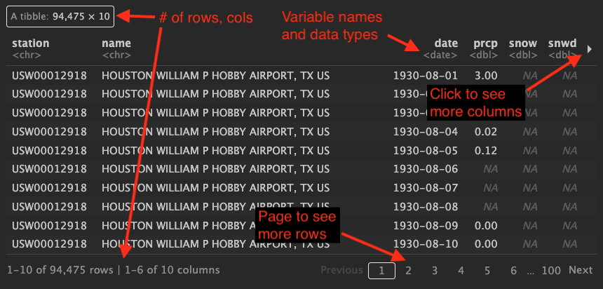
ℹ Specify the column types or set `show_col_types = FALSE` to quiet this message.

We get two outputs here in our notebook:

The R Console pane shows messages about our import.
The second pane shows our data. The data construct here is called a data frame or tibble.

The pipe

To provide some consistency and save from having to use the shift key so much, we are going to run our data through a function called clean_names() after we read it in. As we do this we’ll learn about the “pipe” which moves the result of an object or function into a new function.

Edit your import chunk to add the code below: |> clean_names().

Tip

You can use Cmd+shift+m inside a code block to type a pipe. If you get %>% instead, don’t fret. Keep reading.

read_csv("data-raw/tx.csv") |> clean_names()

Rows: 94503 Columns: 10
── Column specification ────────────────────────────────────────────────────────
Delimiter: ","
chr  (2): STATION, NAME
dbl  (7): PRCP, SNOW, SNWD, TAVG, TMAX, TMIN, TOBS
date (1): DATE

ℹ Use `spec()` to retrieve the full column specification for this data.
ℹ Specify the column types or set `show_col_types = FALSE` to quiet this message.

Our result now comes in two “tabs” for lack of a better word:

The first tab called “R Console” has the output from the read_csv() function.
The second tab called “spec_tbl_df” has output from the clean_names() function.

About clean_names()

The clean_names() function is from the janitor package, and it standardizes the names of our columns, which we call “variables” in R. (Our rows are called “observations”.)

It lowercases all the variable names.
It standardizes the text, removing special characters, etc.
If the variable names have more than one word, it will put an underscore between them: birth_date.

Using clean_names() is a preference and you don’t have to do it. I almost always do. It can save keyboard strokes later and makes it easy to copy/paste the variable names.

About the pipe |>

The pipe is a construct that takes the result of an object or function and passes it into another function. Think of it like a sentence that says “AND THEN” the next thing.

Like this:

I woke up |> 
  got out of bed |>
  dragged a comb across my head

You can’t start a new line with a pipe. If you are breaking your code into multiple lines, then the |> needs to be at the end of a line and the next line should be indented so there is a visual clue it is related to line above it, like this:

read_csv("data-raw/tx.csv") |> 
  clean_names()

It might look like there are no arguments inside clean_names(), but what we are actually doing is passing the imported data frame into it like this:

clean_names(read_csv("data-raw/tx.csv"))

For a lot of functions in R the first argument is “what data are you taking about?” The pipe allows us to say “hey, take the data we just mucked with (i.e., the code before the pipe) and use that in this new function.”

You can see from the nested example that code without the pipe can get confusing. Using the pipe makes our code much more readable.

A rabbit dives into a pipe

The concept of the pipe was first introduced by tidyverse developers in 2014 in a package called magrittr. They used the symbol %>% as the pipe. It was so well received the concept was written directly into base R in 2021, but using the symbol |>. Hadley Wickham’s 2022 rewriting of R for Data Science uses the base R pipe |> by default, so we are too. We configured which version to use in RStudio when we updated preferences.

This switch to |> is quite recent so you will still see %>% used in our training and in documentation online. Assume |> and %>% are interchangeable.

Objects

While we have data printing to our screen, it hasn’t been saved and we can’t reuse it. That’s next.

To save something in our R environment to reuse it, we create an “object”. An object can be made from vector (a list of one or more like items), a data frame (a collection of vectors, like a structured spreadsheet) or even a plot. In short, it is how we save things in our environment (in memory) to reuse later.

By convention we name the object first, then use <- to fill it with our data. Think of it like this: You must have a bucket first before you can fill it with water. The arrow shows you which way the water is flowing.

Edit your import code block to add the tx_raw <- part shown below
Re-run the chunk. Again, Cmd+shift+return will run the entire chunk.

tx_raw <- read_csv("data-raw/tx.csv") |> clean_names()

Rows: 94503 Columns: 10
── Column specification ────────────────────────────────────────────────────────
Delimiter: ","
chr  (2): STATION, NAME
dbl  (7): PRCP, SNOW, SNWD, TAVG, TMAX, TMIN, TOBS
date (1): DATE

ℹ Use `spec()` to retrieve the full column specification for this data.
ℹ Specify the column types or set `show_col_types = FALSE` to quiet this message.

We still get messages about our input
But instead of printing our data to the screen, we have saved it into tx_raw.
If you look at your Environment pane at the top-right of RStudio, you’ll see your saved object listed there.

Tip

You can use Option+i in a code chunk to type in <-.

Let’s print the data out again so we can see it.

Edit your import chunk to add two returns after our line of code and then type out our object so it will display again.

tx_raw <- read_csv("data-raw/tx.csv") |> clean_names()

Rows: 94503 Columns: 10
── Column specification ────────────────────────────────────────────────────────
Delimiter: ","
chr  (2): STATION, NAME
dbl  (7): PRCP, SNOW, SNWD, TAVG, TMAX, TMIN, TOBS
date (1): DATE

ℹ Use `spec()` to retrieve the full column specification for this data.
ℹ Specify the column types or set `show_col_types = FALSE` to quiet this message.

tx_raw

Let’s talk about this output a little because there is a lot of useful information here and it looks different in your notebook vs a rendered page.

OYO: Import new data

Here I want you to import weather data from a different state and save it into an object. You can look in the data-raw folder to see the files to choose from, perhaps from your state.

After these directions but before the next headline, add a new code chunk.
Use the read_csv() command to read in your data and run it to make sure it works.
Edit that same chunk to save your data into a new object. Make sure you see it in your Environment tab.
Add a new line with your new object so it will print out so you can see it.
Add some notes in text to tell your future self what you’ve done.

Peeking at data

There are a number of ways to look at your data. We’ll tour through some.

Head, Tail

With head() and tail() you can look at the “top” and “bottom” of your data. The default is to show six lines of data, but you can add an argument to do more.

Where indicated after the ## Peeking headline, add a new chunk.
Start with your tx_raw data and pipe into head() like below.

tx_raw |> head()

As indicated in the Peeking section, add a chunk and get 8 lines from the bottom of your data.

tx_raw |> tail(8)

Glimpse

The glimpse() function allows you to look at your data in another way … to see all the variables and their data types, no matter how many there are.

As indicated in the practice notebook, add a chunk and glimpse your data like below.

tx_raw |> glimpse()

Rows: 94,503
Columns: 10
$ station <chr> "USW00012918", "USW00012918", "USW00012918", "USW00012918", "U…
$ name    <chr> "HOUSTON WILLIAM P HOBBY AIRPORT, TX US", "HOUSTON WILLIAM P H…
$ date    <date> 1930-08-01, 1930-08-02, 1930-08-03, 1930-08-04, 1930-08-05, 1…
$ prcp    <dbl> 3.00, 0.09, NA, 0.02, 0.12, NA, NA, NA, 0.00, 0.00, 0.00, NA, …
$ snow    <dbl> NA, NA, NA, NA, NA, NA, NA, NA, NA, NA, NA, NA, NA, NA, NA, NA…
$ snwd    <dbl> NA, NA, NA, NA, NA, NA, NA, NA, NA, NA, NA, NA, NA, NA, NA, NA…
$ tavg    <dbl> NA, NA, NA, NA, NA, NA, NA, NA, NA, NA, NA, NA, NA, NA, NA, NA…
$ tmax    <dbl> 99, 97, 95, 95, 92, 92, 96, 97, 94, 92, 99, 99, 98, 98, 98, 97…
$ tmin    <dbl> 75, 79, 78, 79, 76, 74, 71, 71, 75, 72, 70, 71, 78, 72, 73, 70…
$ tobs    <dbl> 86, 89, 89, 85, 83, 89, 83, 82, 85, 85, 87, 86, 86, 85, 86, 84…

This is super handy to have because you can see all your variable names in the same screen. I use it all the time.

Summary

The summary() function loops through all your variables and gives you some basic information about them, especially when they are numbers or dates.

At the indicated spot in the notebook, add a chunk and get a summary of your data like this below:

tx_raw |> summary()

   station              name                date                 prcp        
 Length:94503       Length:94503       Min.   :1930-08-01   Min.   : 0.0000  
 Class :character   Class :character   1st Qu.:1959-01-12   1st Qu.: 0.0000  
 Mode  :character   Mode  :character   Median :1980-08-05   Median : 0.0000  
                                       Mean   :1980-06-04   Mean   : 0.1121  
                                       3rd Qu.:2002-03-09   3rd Qu.: 0.0000  
                                       Max.   :2023-09-30   Max.   :12.0700  
                                                            NA's   :1867     
      snow            snwd            tavg            tmax       
 Min.   :0.000   Min.   :0.000   Min.   : 0.0    Min.   : 13.00  
 1st Qu.:0.000   1st Qu.:0.000   1st Qu.:60.0    1st Qu.: 69.00  
 Median :0.000   Median :0.000   Median :73.0    Median : 81.00  
 Mean   :0.003   Mean   :0.004   Mean   :70.2    Mean   : 78.56  
 3rd Qu.:0.000   3rd Qu.:0.000   3rd Qu.:82.0    3rd Qu.: 91.00  
 Max.   :7.800   Max.   :7.000   Max.   :98.0    Max.   :112.00  
 NA's   :15369   NA's   :15463   NA's   :78843   NA's   :16      
      tmin            tobs      
 Min.   :-2.00   Min.   :24.00  
 1st Qu.:47.00   1st Qu.:61.00  
 Median :61.00   Median :72.00  
 Mean   :58.65   Mean   :69.65  
 3rd Qu.:72.00   3rd Qu.:80.00  
 Max.   :93.00   Max.   :99.00  
 NA's   :16      NA's   :91914

This is super useful to get basic stats like the lowest, highest, average and median values.

You can also do this for a specific column, like to check a date range within your data:

tx_raw$date |> summary()

        Min.      1st Qu.       Median         Mean      3rd Qu.         Max. 
"1930-08-01" "1959-01-12" "1980-08-05" "1980-06-04" "2002-03-09" "2023-09-30"

OYO: Peek at your own data

At the place indicated in your practice notebook, use these “peeking” functions to look at the data in your state. At least try glimpse() and summary().

Create or change data

A little later in our analysis we will want to do some calculations in our data based on the year and month of our data. If we were doing this analysis for the first time we might not realize that yet and would end up coming back to this notebook to do this, but we have the knowledge of foresight here.

We’ll use the mutate() function here to create a new column based on other columns. As the name implies, mutate() changes or creates data.

Let’s explain how mutate works first:

# This is just explanatory psuedo code
# You don't need this in your notebook
data |> 
  mutate(
    newcol = new_stuff_from_math_or_whatever
  )

That new value could be arrived at through math or any combination of other functions. In our case, we will be plucking out parts of our date variable to create some other useful variables. The first one we’ll build is to get the “year” from our date.

Build the machine

We are going to build this code chunk piece by piece, like we would if we were figuring it out for the first time. I want you to see the logic of working through a task like this.

Where indicated in ## Mutate section, add a new code chunk to create your date parts.
Type the code I have below and run the chunk. I’ll explain it afterward.

tx_dates <- tx_raw

tx_dates |> glimpse()

Rows: 94,503
Columns: 10
$ station <chr> "USW00012918", "USW00012918", "USW00012918", "USW00012918", "U…
$ name    <chr> "HOUSTON WILLIAM P HOBBY AIRPORT, TX US", "HOUSTON WILLIAM P H…
$ date    <date> 1930-08-01, 1930-08-02, 1930-08-03, 1930-08-04, 1930-08-05, 1…
$ prcp    <dbl> 3.00, 0.09, NA, 0.02, 0.12, NA, NA, NA, 0.00, 0.00, 0.00, NA, …
$ snow    <dbl> NA, NA, NA, NA, NA, NA, NA, NA, NA, NA, NA, NA, NA, NA, NA, NA…
$ snwd    <dbl> NA, NA, NA, NA, NA, NA, NA, NA, NA, NA, NA, NA, NA, NA, NA, NA…
$ tavg    <dbl> NA, NA, NA, NA, NA, NA, NA, NA, NA, NA, NA, NA, NA, NA, NA, NA…
$ tmax    <dbl> 99, 97, 95, 95, 92, 92, 96, 97, 94, 92, 99, 99, 98, 98, 98, 97…
$ tmin    <dbl> 75, 79, 78, 79, 76, 74, 71, 71, 75, 72, 70, 71, 78, 72, 73, 70…
$ tobs    <dbl> 86, 89, 89, 85, 83, 89, 83, 82, 85, 85, 87, 86, 86, 85, 86, 84…

What are doing here is creating a machine of sorts that we will continue to tinker with.

We are creating a new object called tx_dates and then filling it with tx_raw.
We then glimpse the new tx_dates object so we can see all the columns and some of the values.

Right now there is no difference between tx_dates and tx_raw but we’ll fix that. Doing it this way allows us to see all our columns at once with glimpse.

Add on the mutate

Edit your code chunk to add a pipe at the end of the first line, then hit return.
Type in the mutate function, then add a return in the middle so we can add multiple arguments in a clean way.
Add the line yr = year(date) inside the mutate.
Run the code and inspect the bottom of the glimpse.

tx_dates <- tx_raw |> 
  mutate(
    yr = year(date)
  )

tx_dates |> glimpse()

Rows: 94,503
Columns: 11
$ station <chr> "USW00012918", "USW00012918", "USW00012918", "USW00012918", "U…
$ name    <chr> "HOUSTON WILLIAM P HOBBY AIRPORT, TX US", "HOUSTON WILLIAM P H…
$ date    <date> 1930-08-01, 1930-08-02, 1930-08-03, 1930-08-04, 1930-08-05, 1…
$ prcp    <dbl> 3.00, 0.09, NA, 0.02, 0.12, NA, NA, NA, 0.00, 0.00, 0.00, NA, …
$ snow    <dbl> NA, NA, NA, NA, NA, NA, NA, NA, NA, NA, NA, NA, NA, NA, NA, NA…
$ snwd    <dbl> NA, NA, NA, NA, NA, NA, NA, NA, NA, NA, NA, NA, NA, NA, NA, NA…
$ tavg    <dbl> NA, NA, NA, NA, NA, NA, NA, NA, NA, NA, NA, NA, NA, NA, NA, NA…
$ tmax    <dbl> 99, 97, 95, 95, 92, 92, 96, 97, 94, 92, 99, 99, 98, 98, 98, 97…
$ tmin    <dbl> 75, 79, 78, 79, 76, 74, 71, 71, 75, 72, 70, 71, 78, 72, 73, 70…
$ tobs    <dbl> 86, 89, 89, 85, 83, 89, 83, 82, 85, 85, 87, 86, 86, 85, 86, 84…
$ yr      <dbl> 1930, 1930, 1930, 1930, 1930, 1930, 1930, 1930, 1930, 1930, 19…

Do you see the new column added at the end? That is our new column that just has the year from each date. Some notes about this:

Within the mutate I started with the name of the new column first: yr. I called the new variable “yr” instead of “year” because there actually is a year() function that we use in that same line and I don’t want to get confused. FWIW, R wouldn’t care, but we are human.
The year(date) code is using the year() function to pluck those four numbers out of each filed in the date column. Since we are creating a new column to put this in, we aren’t changing our original data at all.

This is the equivalent of adding a new column to a spreadsheet, and then using a formula that builds from other columns in the spreadsheet and then copying it all the way down the sheet.

If you want to see this in a table view, you can highlight just the tx_dates object in the last line of the code chunk and do Cmd+return on your keyboard to print it to your screen. You could then page over to see the new column. I like using glimpse instead so I can see all the columns at once, but it takes some getting used to.

Add more components

We’ll add two more columns to our spreadsheet within the same mutate() function.

Edit your code chunk to add two new arguments to the code chunk as noted below. I explain them after.

tx_dates <- tx_raw |> 
  mutate(
    yr = year(date),
    mn = month(date, label = TRUE),
    yd = yday(date)
  )

tx_dates |> glimpse()

Rows: 94,503
Columns: 13
$ station <chr> "USW00012918", "USW00012918", "USW00012918", "USW00012918", "U…
$ name    <chr> "HOUSTON WILLIAM P HOBBY AIRPORT, TX US", "HOUSTON WILLIAM P H…
$ date    <date> 1930-08-01, 1930-08-02, 1930-08-03, 1930-08-04, 1930-08-05, 1…
$ prcp    <dbl> 3.00, 0.09, NA, 0.02, 0.12, NA, NA, NA, 0.00, 0.00, 0.00, NA, …
$ snow    <dbl> NA, NA, NA, NA, NA, NA, NA, NA, NA, NA, NA, NA, NA, NA, NA, NA…
$ snwd    <dbl> NA, NA, NA, NA, NA, NA, NA, NA, NA, NA, NA, NA, NA, NA, NA, NA…
$ tavg    <dbl> NA, NA, NA, NA, NA, NA, NA, NA, NA, NA, NA, NA, NA, NA, NA, NA…
$ tmax    <dbl> 99, 97, 95, 95, 92, 92, 96, 97, 94, 92, 99, 99, 98, 98, 98, 97…
$ tmin    <dbl> 75, 79, 78, 79, 76, 74, 71, 71, 75, 72, 70, 71, 78, 72, 73, 70…
$ tobs    <dbl> 86, 89, 89, 85, 83, 89, 83, 82, 85, 85, 87, 86, 86, 85, 86, 84…
$ yr      <dbl> 1930, 1930, 1930, 1930, 1930, 1930, 1930, 1930, 1930, 1930, 19…
$ mn      <ord> Aug, Aug, Aug, Aug, Aug, Aug, Aug, Aug, Aug, Aug, Aug, Aug, Au…
$ yd      <dbl> 213, 214, 215, 216, 217, 218, 219, 220, 221, 222, 223, 224, 22…

This added two new columns to our date, one for the month and one for “day of the year”.

The month(date, label = TRUE) function gives us what is called an “ordered factor” with an abbreviation of our month name. Factors are text strings that understand order, so this field knows that “Jan” comes before “Feb” instead of ordering things alphabetically. If this were a string <chr> then “Apr” would come first when we sorted it. If we didn’t include the part , label = TRUE then we would’ve gotten a number fo the date, like 8 for August.
The yday(date) function is getting us how many days into the year this date falls. So if it were February 1st it would give us “32” since there are 31 days in January. This is probably overkill to create this, but I have a challenge for you later that needs it.

About Lubridate

The functions we used above to get those date components comes from the lubridate package, which gets loaded with our tidyverse library. It is a package designed to ease the friction of working with dates (get it?), which can be a challenge in programming. You can use it to convert text into dates, get date components, adjust time zones and all kinds of things. I use the cheatsheet from this package a lot, usually to “parse date-times” or “get and set components”.

OYO: Create new date compoents

On your own, create date components with your state’s data like we did above. Follow the same steps to build the machine like we did in the example instead of copy/pasting.

Recoding values

In our weather data we have the name column that has the name of the station the reading came from. Those names are pretty long and will get unwieldy later, so let’s create more simple names for the cities, like “Austin”, “Houston” and “Dallas”.

Find distinct values

It would be nice to see the station names easily so we can spell them correctly. We’ll use a function called distinct() to find the unique values for name.

In the ## Recoding values section of your notebok, add a code chunk after the prompt about distinct.
Add the code below and run it.

tx_dates |> distinct(name)

We are taking our data AND THEN finding the “distinct” values in our name column.

We don’t need to save this into a new object or anything. It’s just to help us copy/paste the names of the stations in the next step.

Use mutate to recode

Now we’ll create a new column called city that we build based off the original names above. We use a more complicated version of mutate to do this because in the end we are creating new data.

In the interest of time we’ll provide the finished code with an explanation vs building it piece by piece.

Add a new code chunk for the recode.
Use the copy-to-clipboard button (top right of chunk) to copy the code then paste it into your chunk and run it.

1tx_names <- tx_dates |>
  mutate(
2    city = recode(
3      name,
4      "HOUSTON WILLIAM P HOBBY AIRPORT, TX US" = "Houston",
      "AUSTIN CAMP MABRY, TX US" = "Austin",
      "DALLAS FAA AIRPORT, TX US" = "Dallas"
    )
  )

5tx_names |> glimpse()

1: We start with our new object and then start filling it with our tx_dates data. We pipe into the mutate on the next line.
2: Inside the mutate function we start with the name of the new column, city, and then set that equal to the values that come from our recode() function.
3: The first argument of recode is what column we are looking into for our original values. For us this is the name column.
4: For each line here, we start with our existing value (which we get from the step above) and then set it to our new value. (This construction is counter to the way R normally works where we usually put our new thing before the old thing.)
5: On the last line we glimpse our new object so we can see if it worked.

Rows: 94,503
Columns: 14
$ station <chr> "USW00012918", "USW00012918", "USW00012918", "USW00012918", "U…
$ name    <chr> "HOUSTON WILLIAM P HOBBY AIRPORT, TX US", "HOUSTON WILLIAM P H…
$ date    <date> 1930-08-01, 1930-08-02, 1930-08-03, 1930-08-04, 1930-08-05, 1…
$ prcp    <dbl> 3.00, 0.09, NA, 0.02, 0.12, NA, NA, NA, 0.00, 0.00, 0.00, NA, …
$ snow    <dbl> NA, NA, NA, NA, NA, NA, NA, NA, NA, NA, NA, NA, NA, NA, NA, NA…
$ snwd    <dbl> NA, NA, NA, NA, NA, NA, NA, NA, NA, NA, NA, NA, NA, NA, NA, NA…
$ tavg    <dbl> NA, NA, NA, NA, NA, NA, NA, NA, NA, NA, NA, NA, NA, NA, NA, NA…
$ tmax    <dbl> 99, 97, 95, 95, 92, 92, 96, 97, 94, 92, 99, 99, 98, 98, 98, 97…
$ tmin    <dbl> 75, 79, 78, 79, 76, 74, 71, 71, 75, 72, 70, 71, 78, 72, 73, 70…
$ tobs    <dbl> 86, 89, 89, 85, 83, 89, 83, 82, 85, 85, 87, 86, 86, 85, 86, 84…
$ yr      <dbl> 1930, 1930, 1930, 1930, 1930, 1930, 1930, 1930, 1930, 1930, 19…
$ mn      <ord> Aug, Aug, Aug, Aug, Aug, Aug, Aug, Aug, Aug, Aug, Aug, Aug, Au…
$ yd      <dbl> 213, 214, 215, 216, 217, 218, 219, 220, 221, 222, 223, 224, 22…
$ city    <chr> "Houston", "Houston", "Houston", "Houston", "Houston", "Housto…

Check our work

Since we can’t see all the cities, it is a good idea to check our data to make sure this worked the way we wanted. We can use the distinct() function again but with both name and city.

Add a new chunk in the indicated place.
Add the code to check your results using distinct on name and city.

tx_names |> distinct(name, city)

Looks good.

OYO: Recode station names for your state

We might be pressed for time by this point, but if possible recode your own state’s data with the proper city. Check your work with distinct, as well.

Select columns

Different weather stations can offer different data, and we are just concerned with some specific variables in or data. We can use the select() command to keep or drop columns.

To make decisions what to keep, we would normally spend time with the documentation for the data to make sure we know what is what.

In the interest of time, I’ve done that for you and I’ve made a list. In short we are saving the date, rain, snow and high/low temperature values, plus the columns we created. We don’t need TOBS or TAVG, and in some states they have others we don’t need.

Also in the interest of time, we’ll copy/paste this instead of typing it all in.

In the ## Select columns section of your notebook, add a code chunk.
Use the copy-to-clipboard button to copy this code and paste it into your chunk. Run it.

Explanations follow.

1tx_tight <- tx_names |>
  select(
2    city,
    date,
3    rain = prcp,
    snow,
    snwd,
    tmax,
    tmin,
    yr,
    mn,
    yd
  )

4tx_tight |> glimpse()

1: We start with our new object and pour into it our tx_names data with its piped changes.
2: Inside select we list the variables we want to keep in the order we want them.
3: For the prcp column, we are also renaming the variable to the more familiar rain. It’s easier to type. In typical R fashion the new name comes first.
4: Lastly we glimpse the data so we can check if we got what we wanted.

Rows: 94,503
Columns: 10
$ city <chr> "Houston", "Houston", "Houston", "Houston", "Houston", "Houston",…
$ date <date> 1930-08-01, 1930-08-02, 1930-08-03, 1930-08-04, 1930-08-05, 1930…
$ rain <dbl> 3.00, 0.09, NA, 0.02, 0.12, NA, NA, NA, 0.00, 0.00, 0.00, NA, NA,…
$ snow <dbl> NA, NA, NA, NA, NA, NA, NA, NA, NA, NA, NA, NA, NA, NA, NA, NA, N…
$ snwd <dbl> NA, NA, NA, NA, NA, NA, NA, NA, NA, NA, NA, NA, NA, NA, NA, NA, N…
$ tmax <dbl> 99, 97, 95, 95, 92, 92, 96, 97, 94, 92, 99, 99, 98, 98, 98, 97, 9…
$ tmin <dbl> 75, 79, 78, 79, 76, 74, 71, 71, 75, 72, 70, 71, 78, 72, 73, 70, 7…
$ yr   <dbl> 1930, 1930, 1930, 1930, 1930, 1930, 1930, 1930, 1930, 1930, 1930,…
$ mn   <ord> Aug, Aug, Aug, Aug, Aug, Aug, Aug, Aug, Aug, Aug, Aug, Aug, Aug, …
$ yd   <dbl> 213, 214, 215, 216, 217, 218, 219, 220, 221, 222, 223, 224, 225, …

OYO: Select

Again, if we have time you could do the same for your state.

Export your data

After all that, we finally have the data the way we want it. I do all this work in a separate notebook like this so I don’t have to rerun all the steps when I’m doing analysis (tomorrow!). It is not unusual that during my analysis I come back to this cleaning notebook, fix things and then rerun all the code. That way the fixes are available to all other notebooks using the data.

OK, how to do we get this data out? We’ll use another readr function called write_rds() to save our data to our computer. We use the .rds file (which stands for “R data store”?) because unlike CSVs it saves all our data types. That’s often the purpose of cleaning to fix data types like converting text to a date, or a ZIP code to text.

In the ## Export your data section of your notebook add a new code chunk.
Take your most recent object and pipe it into write_rds() as indicated below.
As you type in the path (inside the quotes) note you can type a few letters and then use tab to complete the path. Write the path for to the data-processed folder and name the file tx_clean.rds, as indicated below.

tx_tight |> write_rds("data-processed/tx_clean.rds")

OYO: Write out your data

Use the same methods as above to write out your state’s data.

Check your notebook

Last thing … we haven’t talked yet about the projects, Quarto and rendering notebooks, but let’s take a brief moment to do two things to make sure our notebooks are working properly.

Go under the Run menu and choose Restart R and Clear Output. This cleans out everything in your notebook.
Go back under Run and choose Run All. This will run all the chunks in your notebook from the top to the bottom.
Check closely through the whole thing for errors. If you have them, you might have feedback in your Console, and in your notebook the code chunk will have a red bar along the left edge.

If there are errors you’ll need to fix them. It is not unusual, especially if you are going up and down the notebook as you work.

Render the notebook

Now that everything is working, you can click the Render button at the top of the notebook RStudio will format your notebook as an HTML page and how it in your Viewer in bottom-right pane.

You’ll notice that rendered version has navigation that can get you to other notebooks in this project, including these lessons you’ve been reading. We’ll talk about how to set these projects up later.

Goals of this lesson

Open the practice file

Packages and libraries

Functions

Importing data

More about readr

The pipe

About clean_names()

About the pipe |>

A rabbit dives into a pipe

Objects

OYO: Import new data

Peeking at data

Head, Tail

Glimpse

Summary

OYO: Peek at your own data

Create or change data

Build the machine

Add on the mutate

Add more components

About Lubridate

OYO: Create new date compoents

Recoding values

Find distinct values

Use mutate to recode

Check our work

OYO: Recode station names for your state

Select columns

OYO: Select

Export your data

OYO: Write out your data

Check your notebook

Render the notebook