```{r}
#| label: setup
#| message: false

library(tidyverse)
```Data Wrangling
FIRST DRAFT DONE. NEED TO CHECK AGAINST SOLUTIONS. THEN MAKE PRACTICE FILE.
Goals of this lesson
For this lesson we’ll learn about data wrangling functions, many of them from dplyr. These are the functions that are much like you do in spreadsheets, like filtering, pivoting and the like. Most of these skills are necessary to prepare data before you make charts.
Function we will learn about include: arrange(), filter(), slice(), group_by() and summarize().
We’ll use these to find several findings from our data, including:
- The coldest and warmest days
- The rainiest and snowiest days
- Years with most snow days
- Years with most 100+ days
- Years with most rain
- Earliest day to reach 100+ each year
To perhaps avoid some confusion we’ll use just the Texas data for this lesson.
(You theoretically could use a different state, but would need to adjust your code to import the right data, use valid cities, etc.)
Clean up our workspace
Again I have a practice notebook ready for you to fill in to keep you on track. Let’s open the file and clean up our environment before we get going.
- Open your
chjr-part1project if it isn’t already. - Open the file
practice-day1-analysis.qmd. - Under run, choose “Restart R and Clear Output”.
- Check your Enfironment tab. If there is anything listed there, click on the broom icon to clear it out.
We do this so we don’t have any leftovers from our previous notebook. Each notebook should run independently. That’s also necessary to Render pages within a project.
Add your setup chunk
I’m going to include the whole setup chunk code here again so you get the execution options.
We only need the tidyverse library for this one.
Import our cleaned data
Now to reap the benefit our the hard work from last lesson, let’s import our cleaned data.
- In the import section of the notebook, add a code chunk.
- Add the
read_rds()function below and fill out the path to your cleaned data, as indicated. - Save that data into a new object called
tx_clean.
tx_clean <- read_rds("data-processed/tx_clean.rds")Arrange
The arrange() function is what we use to sort our data. We can use this function to find a couple of answers were looking for, like what are the hottest and coldest days in our data.
The function is pretty simple, just feed it the data (usually from a pipe) and then add the column you want to sort on. By default it is in “ascending” order: low to high or alphabetically. If you want the opposite (and journalists usually do) you have to wrap the column in another function, desc().
- In the arrange section, add a code chunk for the “Coldest day” section.
- Start with your data, the pipe into
arrange()and add thetmin()column. - Run the chunk so you can see the result. Note the data is ordered by the tmin column, but it’s hard to see. Let’s add a
select()function to focus on what we care about. - Pipe into
select()adding the city, date and tmin columns.
tx_clean |>
  arrange(tmin) |>
  select(city, date, tmin)
Glad I as not in Austin in 1949. Now to find the hottest days.
- After the “Hottest day” header add a new code chunk.
- Use arrange to find the highest
tmaxvalue. Run the chunk to make sure it worked. - Use select to clean up the fields.
tx_clean |>
  arrange(desc(tmax)) |>
  select(city, date, tmax)
Ugh, I was in Austin in 2011.
OYO: Most rain
Using the same tools, find:
- The days with the most rain
- The days with the most snow
Filter
We use the filter() function when we want to specify rows based on a condition. This is the equivalent of clicking on the Filter tool in Excel and choosing values to keep or exclude, but we do it with code that can be fixed and repeated.
We’ll use this function to build to some of our answers, like which years had the most 100+ degree days. We need to work on this skill here first, as there are nuances.
The function works like this:
# this is psuedo code. don't add it
data |>
  filter(variable comparison value)

# example
tx_clean |>
  filter(city == "Austin")
The filter() function typically works in this order:
- What is the variable (or column) you are searching in.
- What is the comparison you want to do. Equal to? Greater than?
- What is the observation (or value in the data) you are looking for?
Note the two equals signs == in our Austin example above. It is important to use two of them when you are asking if a value is “true” or “equal to”, as a single = typically means you are assigning a value to something.
Comparisons: Logical tests
There are a number of these logical tests for the comparison:
| Operator | Definition |
|---|---|
| x < y | Less than |
| x > y | Greater than |
| x == y | Equal to |
| x <= y | Less than or equal to |
| x >= y | Greater than or equal to |
| x != y | Not equal to |
| x %in% c(y,z) | In a group |
| is.na(x) | Is NA (missing values) |
| !is.na(x) | Is not NA |
Where you apply a filter matters. If we want to consider only certain data before other operations, then we need to do the filter first. In other cases we may filter after all our calculations just to clean up the result to show rows of interest.
Single condition
Let’s find days that are 100+.
- In the
## Filtersection in the part about 100+ days, add a code chunk. - Start with the data, the pipe into filter
- For the condition, look in the
tmaxcolumn using>=to find values “greater or equal to”100 - Run the code to make sure it works.
- Use
select()to focuse on the variables of interest.
tx_clean |>
  filter(tmax >= 100) |>
  select(city, date, tmax)
Multiple “and” conditions
OK, that’s fine, but our list is not long enough to see the days in Dallas. Let’s do this again, but add a second condition to test. When you use a comma , or ampersand & between conditions, both conditions must be true to keep the rows.
- In the Dallas 100+ section, start a new code chunk.
- Do the same code as above and run it to make sure it still works.
- Use a comma after the first condition to add a second one:
city == "Dallas".
tx_clean |>
  filter(tmax >= 100, city == "Dallas") |>
  select(city, date, tmax)
Multiple “or” conditions
But what if we have an “either or” case where one of two conditions could be true. This would be the case if we wanted to find days where it either a) snowed that day, or b) there was snow left on the ground from a previous day. This is a true snow day, right?
You can use the | operator for an “or” condition. That character is the shift of the \ key just above your return/enter key.
- In the section about snow days, add a chunk.
- Add the code, but run after adding the first condition, before you add the second, so you can compare them when you are done.
tx_clean |>
  filter(snow > 0 | snwd > 0) |>
  select(city, date, snow, snwd)
But I need “and” and “or”
You can mix “and” and “or” conditions, but note the order of them might matter depending on what you are doing.
OYO: Real snow days in Dallas
In your notebook, start with the snow days we had above, but add a new condition to it that
Filtering text
Our data here doesn’t lend itself well to explaining this, but we can use filter to find parts of words as well. There are many ways, but the one I use the most is str_detect().
tx_clean |>
1  filter(str_detect(city, "st")) |>
distinct(city)- 1
-
Inside the filter, we start with
str_detect(). The first argument it needs is which column in our data to look at, so we fed itcity. The second argument (after a comma) is the string of text we are looking for in the column, which isstin our case.
The code above found both “Houston” and “Austin” because they have “st” in them. It didn’t capture “Dallas”.
Slice
Another way to pick out specific rows of data based on a condition is to use slice variables like slice_max(), slice_min(). I mainly want to show this so you can understand our next function better.
Let’s use slice_min() to find the coldest day in our data.
- In the slice section of the notebook about coldest day, add the following:
tx_clean |>
  slice_min(tmin) |>
  select(city, date, tmin)
We get one result, the coldest day in the data. But what if we want the coldest day for each city? We will introduce group_by() to solve that.
Group by
The group_by() function goes behind the scenes to organize your data into groups, and any function that follows it gets executed within those groups.
The columns you feed into group_by() determine the groups. If we do group_by(city) then all the “Austin” rows are grouped together, then all the “Dallas” rows, then all the “Houston” rows.
I sometimes think of these groups as piles of data, separate from each other. We would have three piles of date, one for each city. Functions that follow happen independently on each pile.
Group and slice
If we add our group_by(city) before slice, then it works within each group. Like this:
tx_clean |>
  group_by(city) |>
  slice_min(tmin) |>
  select(city, date, tmin)
Look at the difference in this result. Now we get a result for each city, because the rows we “grouped” the data before performing the slice. Since there are three cities, we get three results.
Multiple groupings
We can also group by multiple columns. What that does is create a group (or pile!) of data for each matching combination of values.
So, if we group_by(city, yr) then we will get a pile for each year of Austin (85 piles because there are 85 years of data for Austin), then a pile for each year in Houston, etc.
If we were to find the hottest day in each of those piles, it would look like this:
- Create a new chunk and add this to your notebook.
- Try it with and without the
distinct()at the end and think about why you got those results.
tx_clean |>
  group_by(yr, city) |>
  slice_max(tmax) |>
  select(city, tmax) |>
  distinct()
Adding missing grouping variables: `yr`I added distinct the distinct() there to remove some ties where there were multiple days in a year with that high temperature.
Summarize
While slice is nice, we really went through this exercise to understand group_by so we can use it with summarize, which allows us to summarize data much like a pivot table in Excel.
Tip
summarise() and summarize() are the same function. The creator of tidyverse is from New Zealand so he has both spellings. I tend to use them both by whim, though the “s” version comes first in type-assist.
If there are no group_by variables, the output will be a single row summarizing all observations in the input. If we have groups, it will contain one column for each grouping variable and one column for each summary statistic we specify.
Let’s do one without groups.
- In the Summarize section, add the following chunk and code.
tx_clean |>
  summarize(
    e_date = min(date),
    l_date = max(date),
    cnt = n()
  )
We have no groups here, so we just get the stats we as for … the earliest date in our data, the latest date in our data and the number of rows.
Add city as a group
- Just use the copy-to-clipboard tool to add this to your notebook and run it to see it.
tx_clean |>
1  group_by(city) |>
  summarise(
    e_date = min(date),
    l_date = max(date),
    cnt = n()
)- 1
- This is where we add the group.
Add both city and yr as a group
tx_clean |>
1  group_by(city, yr) |>
  summarise(
    e_date = min(date),
    l_date = max(date),
    cnt = n()
)- 1
- This is where we add the second group to get both city and yr.
`summarise()` has grouped output by 'city'. You can override using the
`.groups` argument.
Common summarize stats
There are a number of statistics we can find about our data within summarize.
n()counts the number of rowsn_distinct()counts the number of distinct values in the columnmin()gives the smallest valuemax()gives the largest value
Some math operators might need the argument na.rm = TRUE to ignore NA (empty) values.
sum()adds values together.mean()gives the mean (or average) value.median()gives the median or middle value
There are other useful ones in the summarise documentation.
Group and summarize: Count
A very typical workflow to answer a data-driven question is to count records. Often the logic is to:
- Do we need to consider all the data or just some of it?
- Group the records by variables of interest, like categories or dates.
- Count the number of records in each group.
We’ll use these general steps to answer this question: What years have had the most 100+ degree days. We’ll start with Austin with careful consideration, then generally show how do it for all the cities.
Here are the steps I used to do this, along with my though process. In some cases I’m editing the code as I go along but all we show is the end result below.
- I started with a new code chunk with the
tx_cleandata. - I then filtered it to Austin and ran it to check it. I saved that result into a new object,
atx. - I added a line that used
summary()to check the dates of theatxdata. It looks like the data starts in June 1938 and there could have been days before that that were 100, so I amended my filter to cut out 1938. The latest date is Sept. 30. 2023. Since this is our current year and there are typically few 100+ days in October, I’ll keep this year, but I’ll note it if I use this in a chart. - I glimpse it again just for convenience to see the column names.
Here is the code:
# get Austin data
atx <- tx_clean |> filter(city == "Austin", yr > 1938)

# check dates
atx$date |> summary()
Min. 1st Qu. Median Mean 3rd Qu. Max.
"1939-01-01" "1960-03-09" "1981-05-16" "1981-05-16" "2002-07-23" "2023-09-30" # peek
atx |> glimpse()Rows: 30,954
Columns: 10
$ city <chr> "Austin", "Austin", "Austin", "Austin", "Austin", "Austin", "Aust…
$ date <date> 1939-01-01, 1939-01-02, 1939-01-03, 1939-01-04, 1939-01-05, 1939…
$ rain <dbl> 0.00, 0.00, 0.01, 0.14, 0.00, 0.00, 0.00, 0.12, 0.41, 0.00, 0.34,…
$ snow <dbl> 0, 0, 0, 0, 0, 0, 0, 0, 0, 0, 0, 0, 0, 0, 0, 0, 0, 0, 0, 0, 0, 0,…
$ snwd <dbl> 0, 0, 0, 0, 0, 0, 0, 0, 0, 0, 0, 0, 0, 0, 0, 0, 0, 0, 0, 0, 0, 0,…
$ tmax <dbl> 69, 73, 74, 73, 70, 72, 72, 69, 73, 66, 58, 49, 54, 58, 53, 55, 6…
$ tmin <dbl> 32, 37, 56, 49, 41, 39, 52, 54, 53, 48, 46, 43, 35, 42, 34, 29, 4…
$ yr <dbl> 1939, 1939, 1939, 1939, 1939, 1939, 1939, 1939, 1939, 1939, 1939,…
$ mn <ord> Jan, Jan, Jan, Jan, Jan, Jan, Jan, Jan, Jan, Jan, Jan, Jan, Jan, …
$ yd <dbl> 1, 2, 3, 4, 5, 6, 7, 8, 9, 10, 11, 12, 13, 14, 15, 16, 17, 18, 19…With my prepped data I can now do my calculations:
- I start with the
atxdata and filter to get days wheretmaxwas 100+. I Run the chunk to check it. - Then I grouped the records by
yr. - Then I summarize to get the count using n(), but with a descriptive column name,
hot_days. - Then I arranged the results to show the most
hot_daysat the top. - Then I added a filter to cut off the list at a logical place, years with 50 days or more.
atx |>
  filter(tmax >= 100) |>
  group_by(yr) |>
  summarize(hot_days = n()) |>
  arrange(desc(hot_days)) |>
  filter(hot_days >= 50)
Here is what that looks like if I try to do it with all the cities. The difference here is I’m not taking as much care with the dates so there might be partial years that are undercounted, but they should at least be lower.
tx_clean |>
  filter(tmax >= 100) |>
  group_by(yr, city) |>
  summarize(hot_days = n()) |>
  arrange(desc(hot_days)) |>
  filter(hot_days >= 30)
`summarise()` has grouped output by 'yr'. You can override using the `.groups`
argument.Apparently the Houston Hobby Airport just doesn’t have that many 100+ degree days compared to Austin and Dallas. That humidity, though …
OYO: Most snow days by city each year
If there is time, you could try to do something similar to count the number of days with it snowed.
Group and Summarize: Math
The next question we want to answer: In each city, which years had the most rain and which had the least? Let’s walk through our questions againL
Do we need to consider all the data?
In this case we definitely want only whole years. We calculated the first date of all the data earlier, and it looks like we’ll have to start with 1940. We’ll also lop off 2023.
Do we need to consider our data in any groups?
We need to add together values in each city and year, so Austin for 1940, then ’41, etc. We’ll group our data by city and yr.
What do we need to calculate?
We need to add together the inches of rain, so we can sum() the rain column.
Work through this in your practice notebook step by step:
- In the “Group and Summarize: Math” section, add a code chunk.
- Start with our data, then filter it to start after 1939 and before 2023. Run the chunk to make sure it works. You might even pipe into a
slice_max()to test if it worked (but then remove it after you have checked.) - Group your data by
cityandyr. - Summarize your data using
sum()on theraincolumn. You probably have to add an argumentna.rm = TRUEto make this work because some days there were no rain andsum()doesn’t know what to do with those blank values. - Arrange the values first by city, then by the summed rain in descending order.
- Save your result into an object and then print it back out so you can see it.
tx_yr_rain <- tx_clean |>
  filter(yr > 1939, yr < 2023) |>
  group_by(city, yr) |>
  summarise(tot_rain = sum(rain, na.rm = TRUE)) |>
  arrange(city, desc(tot_rain))
`summarise()` has grouped output by 'city'. You can override using the
`.groups` argument.tx_yr_rainAt this point we have all the values, through they are hard to read. Some directions we could take to get more clarity:
- We could take our new object and build new blocks to filter by city and arrange by most or least rain. Six new code chunks. Very clear.
- We could maybe use group and slice_max to find highest values within each city, and then again with slice_min. There is an option to set the number of returns.
- We could plot this on a chart (a lesson for another day!).
Here is the group and slice method where I use the n = argument to set how many records I want in the slice.
tx_yr_rain |>
group_by(city) |>
slice_max(tot_rain, n = 3)Here is the least rain:
tx_yr_rain |>
group_by(city) |>
slice_min(tot_rain, n = 3)OYO: Years with most snow
Try to do the same to fine the years with the most snow in each city.
Working through logic
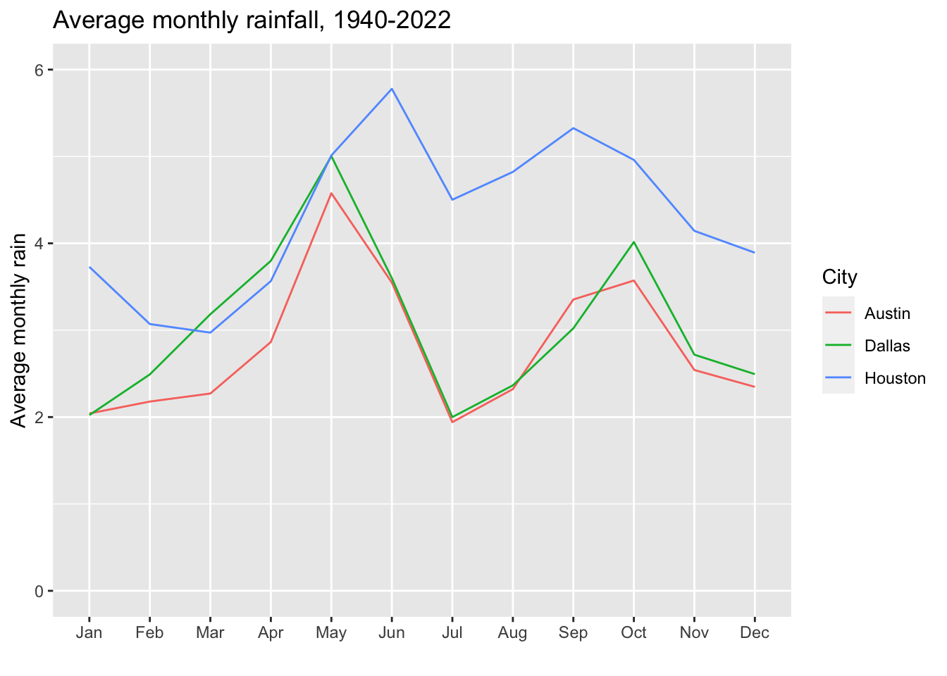
Here is a question that takes a couple of steps to accomplish: What is the average monthly rainfall for each city? i.e., How much rain should we expect each month, based on history?
Do we need to consider all our data? Again, we want just full years, so 1940 through 2022.
Do we need to consider data in groups? This is tricky. We can’t just group by month and get the average because then we would be averaging the rain each day within a month. We have to total the rain within a month for each year, then we can get the average.
What calculations do we need? Kinda answered that in that we need two calculations: One to total the rain within each month/year, and another to get the averages across those months.
We could do the code all in one chunk, but you wouldn’t see the result of the first group and sum, so we’ll do it in two.
tx_mn_yr_rain <- tx_clean |>
1 filter(yr >= 1940, yr <= 2022) |>
2 group_by(city, mn, yr) |>
3 summarize(mn_yr_rain = sum(rain, na.rm = TRUE))- 1
- We filter to get our full years
- 2
- We group by three things so we can add the rain in each city for each month of each year.
- 3
-
We then sum the rain with a nice name. We use
na.rm = TRUEbecause there were cases where the rain value was blank instead of 0.0. Perhaps the station was down? Would need to do some reporting to figure that out.
`summarise()` has grouped output by 'city', 'mn'. You can override using the
`.groups` argument.tx_mn_yr_rain city_avg_rain <- tx_mn_yr_rain |>
1 group_by(city, mn) |>
2 summarise(avg_mn_rain = mean(mn_yr_rain))- 1
- We take the result from above and group now by each city and each month, so we can work with all the “Austin in Jan” to get our average.
- 2
-
Now we can get the average
mean()of those months.
`summarise()` has grouped output by 'city'. You can override using the
`.groups` argument.city_avg_rainAnd to tease you into what is in store for you tomorrow, let’s plot those results:
city_avg_rain |>
  ggplot(aes(x = mn, y = avg_mn_rain, group = city)) +
  geom_line(aes(color = city)) +
  ylim(0,6) +
  labs(
    title = "Average monthly rainfall, 1940-2022",
    x = "", y = "Average monthly rain",
    color = "City"
  )
Challenge: Earliest 100+ day each city
Find the earliest date in each city where it reached at least 100 degrees. Here is a hint: We have the yd field that is the number of days into a year.
What do you want to learn about the weather?
Dream up a question and answer it. Maybe import your own state’s data and find something there. The earliest snowfall. The snowiest month on average. The first freeze. The last freeze. Or more challenge, the average day of the last freeze (i.e., when can I plan my garden!).