3 Billboard Cleaning

This lesson was written by Prof. McDonald and I use macOS.

“If you’re doing data analysis every day, the time it takes to learn a programming language pays off pretty quickly because you can automate more and more of what you do.” – Hadley Wickham, chief scientist at Posit

3.1 Learning goals of this lesson

Practice organized project setup.
Learn a little about data types available to R.
Learn how to download and import CSV files using the readr package.
Introduce the tibble/data frame.
String functions together with the pipe: |> (or %>%).
Learn how to modify data types (date) and select() columns.

Every project in this book is built around a data source that can birth acts of journalism. For this first one we’ll be exploring the Billboard Hot 100 music charts. You’ll use R skills to find the answer to a bunch of questions in the data and then write about it.

3.2 Basic steps of this lesson

Before we get into our storytelling, we have to set up our project, get our data and make sure it is in good shape for analysis. This is pretty standard for any new project. Here are the major steps we’ll cover in detail for this lesson (and many more to come):

Create your project structure
Find the data and (usually) get it onto on your computer
Import the data into your project
Clean up column names and data types
Export cleaned data for later analysis

So this chapter is about collecting and cleaning data. We’ll handle the analysis separately in another chapter. I usually break up projects this way (cleaning vs analyzing) to stay organized and to avoid repeating the same cleaning steps.

3.3 Create a new project

We started a new Quarto website in Chapter 2 so you got this! Here are the basic steps for you to follow:

Launch RStudio if you haven’t already.
Make sure you don’t have an existing project open. Use File > Close project if you do.
Use the +R button to create a project in a New Directory. For project type, choose Quarto Website.
Name the project yourfirstname-billboard and put it in your ~/Documents/rwd folder.

3.3.1 Update index with project description

For our projects, we want to use the index.qmd file (and our resulting website home page) as a description of the project. This is so you, your editor and anyone you share this with can see what this is about.

To save time and such, I’ll supply you with a short project description.

---
title: "Billboard Hot 100"
---

This project is an assignment in the Reporting with Data class at the University of Texas at Austin. 

It is a study of [Billboard Hot 100](https://www.billboard.com/charts/hot-100/) chart data as collected and updated by Christian McDonald in a [Github repo](https://github.com/utdata/rwd-billboard-data). While the archive was compiled through a number of methods, the original source is Billboard Magazine, owned by the Penske Media Corporation. The data dates back to the Hot 100's beginning in August 1958 and is updated weekly, but the end date here will depend on when the user runs the code.

Copy the text above and replace the contents of index.qmd.
Use the Render button or Cmd-Shift-K to render the page.

Important

You want each of your projects to have a description like this, along with details describing the source data, the goals of the project, the findings and perhaps links to stories and graphics published based on the data analysis. If you want to see some excellent examples of these summaries, check out the “Repo” links at Buzzfeed News’ github repo. (RIP Buzzfeed News.)

In the next chapter you’ll return to this page to update it with your findings. For now we’re done with this file so you can close it.

3.3.2 Create directories for your data

Next we are going to create some folders in our project. We’ll use some standard names for consistency and we’ll do this for every project we build.

The first folder is called data-raw. We are creating this folder because we want to keep a pristine version of our original data that we never change or overwrite. This is a core data journalism commandment: Thou shalt not change original data.

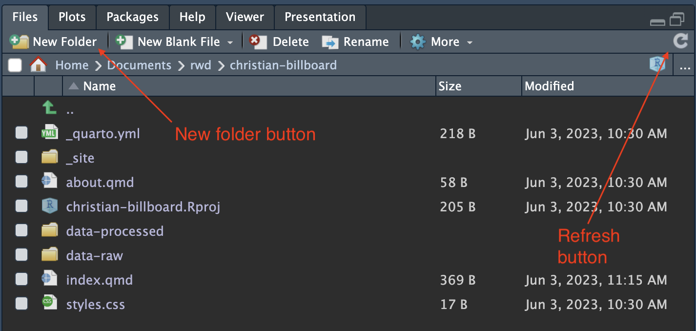
In your Files pane at the bottom-right of RStudio, there is a New Folder icon.

Click on the New Folder icon.
Name your new folder data-raw. This is where we’ll put raw data that we don’t want to overwrite.
Create an additional folder called data-processed. This is were we will write any data we create.

Once you’ve done that, they should show up in the file explorer in the Files pane. Click the refresh button if you don’t see them. (The circlish thing at top right of the screenshot below. You might have to widen the pane to see it.)

Again, we’ll do this with every new project we create:

Create a Quarto website
Update the index with information about the project
Create data-raw and data-processed folders.

3.4 Create our cleaning notebook

We’ll typically use at least three Quarto files in our projects:

The index.qmd that describes the project.
A “Cleaning” notebook where we prepare our data.
An “Analysis” notebook where we pose and answer our data questions.

So let’s create our “Cleaning” notebook.

Use the top left new document button ( a white box with a green + sign) and choose the Quarto Document to start a new notebook.
Set the title to “Cleaning”.
Make sure the Editor choice to use the visual editor is NOT checked. Everything else should be fine.
Click Create. This creates an Untitled document that we still need to save.
Save the new file (Do Cmd-S or look under the File menu or use the floppy disc icon in the tool bar.)
Name the file 01-cleaning.qmd. It should already be set to save in the project folder.

Tip

We named this notebook starting with 01- because we will eventually end up with multiple notebooks that depend on each other and we will need to know the order to run them in the future.

3.5 Update our _quarto.yml

We’ve created our cleaning notebook and it will Render, but it won’t show up in our website navigation yet until we specifically add it. The _quarto.yml config file controls various output options for the “website” that you are creating.

Open the _quarto.yml file.
On the line that now says - about.qmd, replace that text with - 01-cleaning.qmd.

Let’s talk a little about the part of the _quarto.yml file we edited:

website:
  title: "christian-billboard"
  navbar:
    left:
      - href: index.qmd
        text: Home
      - 01-cleaning.qmd

Note the indents and dashes and such are important in YAML files. Under the “parent” line website we have two children, title and navbar. The navbar line has a child of left and that has two children - href and - 01-cleaning.qmd.

When we added the 01-cleaning.qmd file it automatically added that to the nav, and then used the title of the page as word linked in the navigation.

But for the index, we don’t want to use the title of the page. We have to define what we are doing with more detail, hence the href (meaning which page will be linked to) and the text to show in the navigation, Home.

While we are here, we should adjust some other configurations:

For the title: change the value to "Billboard Hot 100". This is the main website name that displays in the navigation bar.
At the bottom of the file on a new line, by itself and starting flush left, add df-print: paged. This makes data we output in our notebooks look more pretty.

Your file should look like this now:

project:
  type: website

website:
  title: "Billboard Hot 100"
  navbar:
    left:
      - href: index.qmd
        text: Home
      - 01-cleaning.qmd

format:
  html:
    theme: cosmo
    css: styles.css
    toc: true

df-print: paged

Make sure you _quarto.yml file is saved.
Go back to your Cleaning notebook and Render it to make there are no errors and that you can see the page in the website navigation.

3.5.1 Describe the goals of the notebook

At the top of the cleaning file after the YAML metadata we’ll want to explain the goals of the notebook and what we are doing.

Add this text to your notebook AFTER the metadata:

## Goals of this notebook

The steps we'll take to prepare our data:

- Download the data
- Import it into our notebook
- Clean up data types and columns
- Export the data for next notebook

We want to start each notebook with a list like this so our future selves and others know what we are trying to accomplish. It’s not unusual to update this list as we work through the notebook.

We will also write Markdown like this to explain each new “section” or goal as we tackle them.

3.6 The setup chunk

In our previous chapter we installed several R packages onto our computer that we’ll use in almost every lesson. There are others we’ll install and use later.

But to use these packages in our notebook (and the functions they provide us) we have to load them using the library() function. We always have to declare these and convention dictates we put it near the top of a notebook so everyone understands what is needed to run our code.

3.6.1 Load the libraries

In your notebook after the goals listing, create a new “section” by adding a headline called “Setup” using Markdown, like this: ## Setup.
After the. headline use Cmd+option+i to insert an R code chunk.
Inside that chunk, I want you to type the code shown below.

I want you to type the code so you can see how RStudio helps you complete the code. It’s something you have to see or do yourself to understand how RStudio helps you type commands, but as you type RStudio will give you valid options you can scroll through and hit tab key to choose.

Here is a gif of me typing in the commands. I’m using keyboard commands like the up and down arrow to make selections, and the tab key to select them. This concept is called code completion.

Here is the code:

```{r}
#| label: setup
#| message: false

library(tidyverse)
library(janitor)
```

3.6.2 About the libraries

A little more about the two packages we are loading here. We use them a lot.

The tidyverse package is actually a collection of packages for data science that are designed to work together. You can see the first time I run the chunk in the gif above that a bunch of libraries were loaded. By loading the whole tidyverse library we get readr functions for importing data, dplyr to manipulate data, lubridate to help work with dates, and ggplot to visualize data. There are more.
The janitor package is not maintained by the same folks at Posit, but it has a couple of useful tools to clean and view data I use a lot, including the clean_names() that we’ll use here.

3.6.3 About the options

I then go back and add some lines at the top of the chunk called execution options. Let’s talk about each line:

We start with #| label: setup which is an execution option to “name” the code chunk. Labeling chunks is optional but useful.
- The chunk label setup is special as it will be run first if it hasn’t already been run.
- When we name a code chunk it creates a bookmark of sorts, which I’ll show you later.
The #| message: false option suppress the message about all the packages loaded since we don’t need to display that in our notebook. I usually only add that for my setup chunk.

Tip: good stopping point

We’ve just done a lot of work setting up our project, and we’re about to get into some important info about our the data we’ll be working with. This would be a good place to take a break if you need to. Seriously, go eat a cookie 🍪

3.7 About the Billboard Hot 100

The Billboard Hot 100 singles charts has been the music industry’s standard record chart since its inception on Aug. 4th, 1958. The rankings, published by Billboard Magazine, are currently based on sales (physical and digital), radio play, and online streaming. The methods and policies of the chart have changed over time.

The data we will use was compiled by Prof. McDonald from a number of sources. When you write about this data (and you will), you should source it as the Billboard Hot 100 from Billboard Magazine, since that is where it originally came from and they are the “owner” of the data.

3.7.1 Data dictionary

Take a look at the current chart. Our data contains many (but not quite all) of the elements you see there. Each row of data (or observation as they are known in R) represents a song and the corresponding position on that week’s chart. Included in each row are the following columns (a.k.a. variables):

CHART DATE: The release date of the chart
THIS WEEK: The current ranking as of the chart date
TITLE: The song title
PERFORMER: The performer of the song
LAST WEEK: The ranking on the previous week’s chart
PEAK POS.: The peak rank the song has reached as of the chart date
WKS ON CHART: The number of weeks the song has appeared as of the chart date

3.7.2 Let’s download our data

Our data is stored on a code sharing website called Github, and it is formatted as a “comma-separated value” file, or .csv. That means it basically a text file where every line is a new row of data, and each field is separated by a comma.

Because it is on the internet and has a URL, we could import it directly into our project from there, but there are benefits to getting the file onto your computer first. The hosted file could change later in ways you can’t control, and you would need Internet access to the file the next time you ran your notebook. If you download the file to keep your own copy, you have more control of your future.

Since this is a new “section” of our cleaning notebook, we’ll note what we are doing and why in Markdown.

Add a Markdown headline ## Downloading data and some text explaining you are downloading data. Add a note about where the data comes from and include a link to the original source. (This way others and future self will know where the data came from.)
Create an R chunk and copy/paste the following inside it. (Given the long URL, go ahead and use the copy icon at the top right of the chunk):

download.file(
  "https://github.com/utdata/rwd-billboard-data/blob/main/data-out/hot100_assignment.csv?raw=true",
  "data-raw/hot100_assignment.csv",
  mode = "wb"
)

Let’s explain about this:

This download.file() code is a function, or a bit of code that has been written to do a specific task. This one (surprise!) downloads files from the internet. As a function, it has some “arguments”, which are expected pieces of information that the function needs to do its job. Sometimes we just enter the arguments in the order that the function expects them, like we do here. Other times we will give it the kind of argument like mode = "w". You can search for documentation about functions in the Help tab in the bottom-right pane of RStudio.

In this case, we are supplying three arguments:

The first is the URL of the file you are downloading. Note that this is in quotes.
The second is the location where we want to save the file, and what want to name it. We call this a “path” and you can see it looks a lot like a URL. This path is in relation to the document we are in, so we are saying we want to put this file in the data-raw/ folder with a name of hot100_assignment.csv, but it is really one path: data-raw/hot100_assignment.csv.
The third argument mode = "w" gets into the weeds a little, but it helps Windows computers understand the file.

trying URL 'https://github.com/utdata/rwd-billboard-data/blob/main/data-out/hot100_assignment.csv?raw=true'
Content type 'text/plain; charset=utf-8' length 18364249 bytes (17.5 MB)
==================================================
downloaded 17.5 MB

That’s not a small file at 17 MB and 300,000 rows, but it’s not a huge one, either.

You can check that this worked by going to your Files tab and clicking on the data-raw folder to go inside it and see if the file is there. To return out of the folder, click on the two dots to the right of the green up arrow.

3.7.3 Comment the download code

Important

The Hot 100 data updates each week. We’ll not download it again so our results don’t change mid-analysis!

Now that we’ve downloaded the data to our computer, we don’t need to run this line of code again unless we want to update our data from the source. We can “comment” the code to preserve it but keep it from running again if we re-run our notebook (and we will).

Above your code chunk, write in Markdown a note to your future self that you commented the download for now.
Inside your code chunk, highlight the lines of code that include the download.file() function, then go under the Code menu to Comment/Uncomment Lines. (Note the keyboard command there Cmd-Shift-C, as it is another useful one!)

Adding comments in programming is a common thing and every programming language has a way to do it. It is a way for the programmer to write notes to their future self, colleagues or — like in this case — comment out some code that you want to keep, but don’t want to execute when the program is run.

We write most of our “explaining” text outside of code chunks using a syntax called Markdown. Markdown is designed to be readable as written, but it is given pretty formatting when “printed” as a PDF or HTML file.

But, sometimes it makes more sense to explain something right where the code is being executed. If you are inside a code chunk, you start the comment with one or more hashes #. Any text on that line that follows won’t be executed as code.

Warning

Yes, it is confusing that in Markdown you use hashes # to make headlines, but in code chunks you use # to make comments. We’re essentially writing in two languages in the same document.

3.8 Import the data

Now that we have the data on our computer, let’s import it into our notebook so we can see it.

Since we are doing a new thing, we should again note what we are doing.

Add a Markdown headline: ## Import data
Add some text to explain that we are importing the Billboard Hot 100 data.
After your description, add a new code chunk (Cmd+Option+i).

We’ll be using the read_csv() function from the tidyverse readr package, which is different from read.csv that comes with base R. read_csv() is mo betta.

Inside the function we put in the path to our data, inside quotes. If you start typing in that path and hit tab, it will complete the path. (Easier to show than explain).

Add the following code into your chunk and run it.

read_csv("data-raw/hot100_assignment.csv")

Tip

Note the path to the file is in quotes!

You get two results printed to your notebook.

The first result called “R Console” shows what columns were imported and the data types. It’s important to review these to make sure things happened the way that expected. In this case it noted which columns came in as text (chr), or numbers (dbl). The red colored text in this output is NOT an indication of a problem.

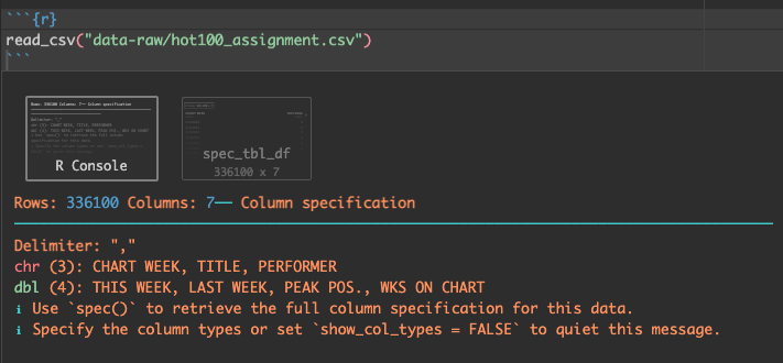
The second result spec_tbl_df prints out the data like a table. The data object is a tibble, which is a fancy tidyverse version of a “data frame”.

Note

I will use the term tibble and data frame interchangably. Think of tibbles and data frames like a well-structured spreadsheet. They are organized rows of data (called observations) with columns (called variables) where every column is a specific data type.

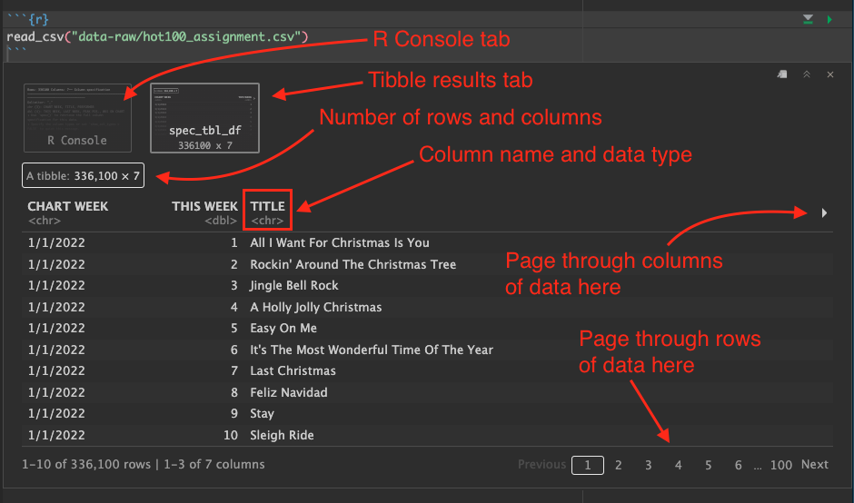
When we look at the data output in RStudio, there are several things to note:

Below each column name is an indication of the data type. This is important.
You can use the arrow icon on the right to page through the additional columns.
You can use the paging numbers and controls at the bottom to page through the rows of data.
The number of rows and columns is displayed.

At this point we have only printed this data to the screen. We have not saved it in any way, but that is next.

3.8.1 Assign our import to an R object

Now that we know how to find our data, we next need to assign it to an R object so it can be a named thing we can reuse. We don’t want to re-import the data over and over each time we need it.

The syntax to create an object in R can seem weird at first, but the convention is to name the object first, then insert stuff into it. So, to create an object, the structure is this:

# this is pseudo code. Don't put it in your notebook.
new_object <- stuff_going_into_object

Think of it like this: You must have a bucket before you can fill it with water. We “name” the bucket, then fill it with data. That bucket is then saved into our “environment”, meaning it is in memory where we can access it easily by calling its name.

Let’s make a object called hot100 and fill it with our imported tibble.

Edit your existing code chunk to look like this. You can add the <- by using Option+- as in holding down the Option key and then pressing the hyphen:

hot100 <- read_csv("data-raw/hot100_assignment.csv")

Run that chunk and several things happen:

We no longer see the result of the data in the notebook because we created an object instead of printing it.
In the Environment tab at the top-right of RStudio, you’ll see the hot100 object listed.
- Click on the blue play button next to hot100 and it will expand to show you a summary of the columns.
- Click on the name hot100 and it will open a “View” of the data in another window, so you can look at it in spreadsheet form. You can even sort and filter it.
Once you’ve looked at the data, close the data view with the little x next to the tab name.

3.8.2 Print a peek to your R Notebook

Since we can’t see the data after we assign it, let’s print the object to our notebook so we can refer to it.

Edit your import chunk to add the last two lines of this, including #:

# create the object, then fill it with data from the csv
hot100 <- read_csv("data-raw/hot100_assignment.csv")

# peek at the data
hot100

You can use the green play button at the right of the chunk, or preferrably have your cursor inside the chunk and do Cmd+Shift+Return to run all lines. (Cmd+Return runs only the current line.)

3.8.3 Glimpse the data

There is another way to peek at the data that I use alot because it is more compact and shows you all the columns and data examples without scrolling: glimpse().

In your existing chunk, edit the last line to add the glimpse() function as noted below.

I’m showing the return here as well. Afterward I’ll explain the pipe: |>.

hot100 <- read_csv("data-raw/hot100_assignment.csv")

# peek at the data
hot100 |> glimpse()

Rows: 341,300
Columns: 7
$ `CHART WEEK`   <chr> "1/1/2022", "1/1/2022", "1/1/2022", "1/1/2022", "1/1/20…
$ `THIS WEEK`    <dbl> 1, 2, 3, 4, 5, 6, 7, 8, 9, 10, 11, 12, 13, 14, 15, 16, …
$ TITLE          <chr> "All I Want For Christmas Is You", "Rockin' Around The …
$ PERFORMER      <chr> "Mariah Carey", "Brenda Lee", "Bobby Helms", "Burl Ives…
$ `LAST WEEK`    <dbl> 1, 2, 4, 5, 3, 7, 9, 11, 6, 13, 15, 17, 18, 0, 8, 25, 1…
$ `PEAK POS.`    <dbl> 1, 2, 3, 4, 1, 5, 7, 6, 1, 10, 11, 8, 12, 14, 7, 16, 12…
$ `WKS ON CHART` <dbl> 50, 44, 41, 25, 11, 26, 24, 19, 24, 15, 31, 18, 14, 1, …

The glimpse shows there are 300,000+ rows and 7 columns in our data. Each column is then listed out with its data type and the first several values in that column.

3.8.4 About the pipe |>

We need to break down this code a little: hot100 |> glimpse().

We are starting with the object hot100, but then we follow it with |>, which is called a pipe. The pipe is a construct that takes the result of an object or function and passes it into another function. Think of it like a sentence that says “AND THEN” the next thing.

Like this:

I woke up |> 
  got out of bed |>
  dragged a comb across my head

You can’t start a new line with a pipe. If you are breaking your code into multiple lines, then the |> needs to be at the end of a line and the next line should be indented so there is a visual clue it is related to line above it, like this:

hot100 |> 
  glimpse()

It might look like there are no arguments inside glimpse(), but what we are actually doing is passing the hot100 tibble into it like this: glimpse(hot100). For almost every function in R the first argument is “what data are you taking about?” The pipe allows us to say “hey, take the data we just mucked with (i.e., the code before the pipe) and use that in this function.”

Tip

There is a keyboard command for the pipe |>: Cmd+Shift+m. Learn that one!

A rabbit dives into a pipe

The concept of the pipe was first introduced by tidyverse developers in 2014 in a package called magrittr. They used the symbol %>% as the pipe. It was so well received the concept was written directly into base R in 2021, but using the symbol |>. Hadley Wickham’s 2022 rewriting of R for Data Science uses the base R pipe |> by default. You can configure which to use in RStudio.

(This switch to |> is quite recent so you might see %>% used in this book. Assume |> and %>% are interchangeable. There is A LOT of code in the wild using the magrittr pipe %>%, so you’ll find many references on Stack Overflow and elsewhere.)

3.9 Cleaning data

Data is dirty. Usually because a human was involved at some point, and we humans are fallible.

Data problems are often revealed when importing so it is good practice to check for problems and fix them right away. We’ll face some of those challenges in this project, but we should talk about what is good vs dirty data.

Good data should:

Have a single header row with well-formed column names.
- Descriptive names are better than not descriptive.
- Short names are better than long ones.
- Spaces in names make them harder to work with. Use and _ or . between words. I prefer _ and all lowercase text.
Remove notes or comments from the files.
Each column should have the same kind of data: numbers vs words, etc.

3.9.1 Cleaning column names

So, given those notes above, we should clean up our column names. This is why we have included the janitor package, which includes a neat function called clean_names()

Edit the first line of your chunk to add a pipe and the clean_names function: %>% clean_names()

hot100 <- read_csv("data-raw/hot100_assignment.csv") %>% clean_names()

# peek at the data
hot100 |> glimpse()

Rows: 341,300
Columns: 7
$ chart_week   <chr> "1/1/2022", "1/1/2022", "1/1/2022", "1/1/2022", "1/1/2022…
$ this_week    <dbl> 1, 2, 3, 4, 5, 6, 7, 8, 9, 10, 11, 12, 13, 14, 15, 16, 17…
$ title        <chr> "All I Want For Christmas Is You", "Rockin' Around The Ch…
$ performer    <chr> "Mariah Carey", "Brenda Lee", "Bobby Helms", "Burl Ives",…
$ last_week    <dbl> 1, 2, 4, 5, 3, 7, 9, 11, 6, 13, 15, 17, 18, 0, 8, 25, 19,…
$ peak_pos     <dbl> 1, 2, 3, 4, 1, 5, 7, 6, 1, 10, 11, 8, 12, 14, 7, 16, 12, …
$ wks_on_chart <dbl> 50, 44, 41, 25, 11, 26, 24, 19, 24, 15, 31, 18, 14, 1, 49…

This function has cleaned up your names, making them all lowercase and using _ instead of periods between words. Believe me when I say this is helpful when you are writing code. It makes type-assist work better and you can now double-click on a column name to select all of it and copy and paste somewhere else. When you have spaces or dashes in an object you can’t double-click on it to select all of it.

3.9.2 Fixing the date

Dates in programming are a tricky data type because they are represented essentially as the number of seconds before/after January 1, 1970. Yes, that’s crazy, but it is also cool because that allows us to do math on them. So, to use our chart_date properly in R we need to convert it from the text into a real date datatype. (If you wish, you can read more about why dates are tough in programming | PDF version.)

Converting text into dates can be challenging, but the tidyverse universe has a package called lubridate to ease the friction. (Get it?).

Since we are doing something new, we want to start a new section in our notebook and explain what we are doing.

In Markdown add a headline: ## Fix our dates.
Add some text that you are using lubridate to create a new column with a real date.
Add a new code chunk. Remember Cmd+Option+i will do that.

We will be changing or creating our data, so we will create a new object to store it in. We do this so we can go back and reference the unchanged data if we need to. Because of this, we’ll set up a chunk of code that allows us to peek at what is happening while we write our code. We’ll do this kind of setup often when we are working out how to do something in code.

Add the following inside your code chunk.
Run the code, and then read through the annotations below.

Tip

This is our first use of annotated code with the circled numbers shown on the right edge of the code block. If you see these, the best way to use the code in the chunk is to a) type it yourself (preferred!), b) to highlight and copy a line without catching the circled number, or c) to use the “Copy to clipboard” icon that shows at the top-right of the code block when you put your cursor over it.

1# part we will build upon
2hot100_date <- hot100
3
4# peek at the result
5hot100_date |> glimpse()

1: I have a comment starting with # to explain the first part of the code.
2: We created a new object (or “bucket”) called hot100_date and we fill it with our hot100 data. Yes, as of now they are exactly the same.
3: I leave a blank line for clarity …
4: Then another comment …
5: Then we glimpse the new hot100_date object so we can see changes as we work on it.

Rows: 341,300
Columns: 7
$ chart_week   <chr> "1/1/2022", "1/1/2022", "1/1/2022", "1/1/2022", "1/1/2022…
$ this_week    <dbl> 1, 2, 3, 4, 5, 6, 7, 8, 9, 10, 11, 12, 13, 14, 15, 16, 17…
$ title        <chr> "All I Want For Christmas Is You", "Rockin' Around The Ch…
$ performer    <chr> "Mariah Carey", "Brenda Lee", "Bobby Helms", "Burl Ives",…
$ last_week    <dbl> 1, 2, 4, 5, 3, 7, 9, 11, 6, 13, 15, 17, 18, 0, 8, 25, 19,…
$ peak_pos     <dbl> 1, 2, 3, 4, 1, 5, 7, 6, 1, 10, 11, 8, 12, 14, 7, 16, 12, …
$ wks_on_chart <dbl> 50, 44, 41, 25, 11, 26, 24, 19, 24, 15, 31, 18, 14, 1, 49…

To be clear, we haven’t changed any data yet. We just created a new object like the old object.

3.9.2.1 Working with mutate()

We are going to use the text of our date field chart_date to create a new converted date. We will use the dplyr function mutate() to do this, with some help from lubridate.

Note

dplyr is the tidyverse package of functions to manipulate data. We’ll use functions from it a lot. Dplyr is loaded with the library(tidyverse) so you don’t have to load it separately.

Let’s explain how mutate works first: Mutate changes every value in a column. You can either create a new column or overwrite an existing one.

Within the mutate function, we name the new thing first (the bucket!) and then fill it with the new value.

# This is just explanatory psuedo code
# You don't need this in your notebook
data |> 
  mutate(
    newcol = new_stuff_from_math_or_whatever
  )

That new value could be arrived at through math or any combination of other functions. In our case, we want to convert our old text-based date to a real date, and then assign it back to the “new” column.

Edit your chunk to add the changes below and run it. I implore you to type the changes so you see how RStudio helps you write it. Use tab completion, etc.

# part we will build upon
1hot100_date <- hot100 |>
2  mutate(
3    chart_date = mdy(chart_week)
  )

# peek at the result
hot100_date |> glimpse()

1: At the end of the first line, we added the pipe |> because we are taking our hot100 data AND THEN we will mutate it. (Remember Cmd-shift-m for the pipe!)
2: Next, we start the mutate() function. If you use type assist and tab completion to type this in, your cursor will end up in the middle of the parenthesis. This allows you to then hit your Return key to split it into multiple lines with proper indenting. We do this so we can more clearly see what inside the mutate … where the real action is going on here. It’s also possible to make multiple changes within the same mutate, and putting each one on their own line makes that more clear.
3: Inside the mutate, we first name our new column chart_date and then we set that equal to mdy(chart_week), which is explained next.

Rows: 341,300
Columns: 8
$ chart_week   <chr> "1/1/2022", "1/1/2022", "1/1/2022", "1/1/2022", "1/1/2022…
$ this_week    <dbl> 1, 2, 3, 4, 5, 6, 7, 8, 9, 10, 11, 12, 13, 14, 15, 16, 17…
$ title        <chr> "All I Want For Christmas Is You", "Rockin' Around The Ch…
$ performer    <chr> "Mariah Carey", "Brenda Lee", "Bobby Helms", "Burl Ives",…
$ last_week    <dbl> 1, 2, 4, 5, 3, 7, 9, 11, 6, 13, 15, 17, 18, 0, 8, 25, 19,…
$ peak_pos     <dbl> 1, 2, 3, 4, 1, 5, 7, 6, 1, 10, 11, 8, 12, 14, 7, 16, 12, …
$ wks_on_chart <dbl> 50, 44, 41, 25, 11, 26, 24, 19, 24, 15, 31, 18, 14, 1, 49…
$ chart_date   <date> 2022-01-01, 2022-01-01, 2022-01-01, 2022-01-01, 2022-01-…

The mdy() function is part of the lubridate package. Lubridate allows us to parse text and then turn it into a real date if we tell it the order of the date values in the original data.

Our original date was something like “7/17/1965”. That is month, followed by day, followed by year.
We use the lubridate function mdy() to say “that’s the order this text is in, now please convert this into a real date”, which properly shows as YYYY-MM-DD. Lubridate is smart enough to figure out if you have / or - between your values in the original text.

If your original text is in a different date order, then you look up what lubridate function you need to convert it. I typically use the cheatsheet in the lubridate documentation. You’ll find them in the PARSE DATE-TIMES section.

Tip

A note about the spacing and indenting of my code above: I strategically used returns to make the code more readable. This code would work the same if it were all on the same line, but writing it this way helps me understand it. RStudio will help you indent properly as you type. (Easier to show than explain.)

3.9.2.2 Check the result!

This new chart_date column is added as the LAST column of our data. After doing any kind of mutate you want to check the result to make sure you got the results you expected, which is why we didn’t just overwrite the original chart_week column. That’s also why we built our code this way with glimpse() so we can see example of our data from both the first and the last column. (We’ll rearrange all the columns in a bit once we are done cleaning everything.)

Check your glimpse returns … did your dates convert correctly?

3.9.3 Arrange the data

Just to be tidy, we want ensure our data is arranged to start with the oldest week and “top” of the chart and then work forward through time and rank.

i.e., let’s arrange this data so that the oldest data is at the top.

Sorting data is not a particularly difficult concept to grasp, but it is one of the Basic Data Journalism Functions, so watch this video:

In R, the sorting function we use is called arrange().

We’ll build upon our existing code and use the pipe |> to push it into an arrange() function. Inside arrange we’ll feed it the columns we wish to sort by.

Edit your chunk to the following to add the arrange() function:

# part we will build upon
hot100_date <- hot100 |> 
  mutate(
    chart_date = mdy(chart_week)
1  ) |>
2  arrange(chart_date, this_week)

# peek at the result
hot100_date |> glimpse()

1: Add the pipe to the end of this line …
2: … and the arrange line

Rows: 341,300
Columns: 8
$ chart_week   <chr> "8/4/1958", "8/4/1958", "8/4/1958", "8/4/1958", "8/4/1958…
$ this_week    <dbl> 1, 2, 3, 4, 5, 6, 7, 8, 9, 10, 11, 12, 13, 14, 15, 16, 17…
$ title        <chr> "Poor Little Fool", "Patricia", "Splish Splash", "Hard He…
$ performer    <chr> "Ricky Nelson", "Perez Prado And His Orchestra", "Bobby D…
$ last_week    <dbl> NA, NA, NA, NA, NA, NA, NA, NA, NA, NA, NA, NA, NA, NA, N…
$ peak_pos     <dbl> 1, 2, 3, 4, 5, 6, 7, 8, 9, 10, 11, 12, 13, 14, 15, 16, 17…
$ wks_on_chart <dbl> 1, 1, 1, 1, 1, 1, 1, 1, 1, 1, 1, 1, 1, 1, 1, 1, 1, 1, 1, …
$ chart_date   <date> 1958-08-04, 1958-08-04, 1958-08-04, 1958-08-04, 1958-08-…

Now when you look at the glimpse, the first record in the chart_date column is from “1958-08-04” and the first in the this_week is “1”, which is the top of the chart.

Just to see this all clearly in table form, we’ll print the top of the table to our screen so we can see it.

Add a line of Markdown text in your notebook explaining your are looking at the table.
Add a new code chunk and add the following.

hot100_date |> head(10)

This just prints the first 10 lines of the data.

Use the arrows to look at the other columns of the data (which you can’t see in the book).

Note

It’s OK that the last_week columns has “NA” for those first rows because this is the first week ever for the chart. There was no last_week.

3.9.3.1 Getting summary stats

Printing your data to the notebook can only tell you so much. Yes, you can arrange by different columns to see the maximum and minimum values, but it’s hard to get an overall sense of your data that way when there is 300,000 rows like we have here. Luckily there is a nice function called summary() that gives you some summary statistics for each column.

Add some Markdown text that you’ll print summary stats of your data.
Add a new R chunk and put the following in and run it

hot100_date |> summary()

  chart_week          this_week        title            performer        
 Length:341300      Min.   :  1.0   Length:341300      Length:341300     
 Class :character   1st Qu.: 26.0   Class :character   Class :character  
 Mode  :character   Median : 51.0   Mode  :character   Mode  :character  
                    Mean   : 50.5                                        
                    3rd Qu.: 75.0                                        
                    Max.   :100.0                                        
                                                                         
   last_week         peak_pos       wks_on_chart      chart_date        
 Min.   :  0.00   Min.   :  1.00   Min.   : 1.000   Min.   :1958-08-04  
 1st Qu.: 23.00   1st Qu.: 13.00   1st Qu.: 4.000   1st Qu.:1974-12-14  
 Median : 47.00   Median : 38.00   Median : 7.000   Median :1991-04-20  
 Mean   : 47.29   Mean   : 40.69   Mean   : 9.288   Mean   :1991-04-19  
 3rd Qu.: 71.00   3rd Qu.: 65.00   3rd Qu.:13.000   3rd Qu.:2007-08-25  
 Max.   :100.00   Max.   :100.00   Max.   :91.000   Max.   :2023-12-30  
 NA's   :32460

These summary statistics can be informative for us. It is probably the easiest way to check what the newest and oldest dates are in your data (see the Min. and Max. returns for chart_date). You get an average (mean) and median for each number, too. You might notice potential problems in your data, like if we had a this_week number higher than “100” (we don’t).

3.9.3.2 Note the max date

Since this data updates each week, it is a good idea to note in your notebook what is the most recent chart date. You can find that as the Max. value for chart_date in your summary. You’ll need this value when you write your story.

3.9.4 Selecting columns

Now that we have the fixed date column, we don’t need the old chart_week version that is text. We’ll use this opportunity to discuss select(), which is another concept in our Basic Data Journalism Functions series, so watch this:

In R, the workhorse of the select concept is the function called — you guessed it — select(). In short, the function allows us to choose a subset of our columns. We can either list the ones we want to keep or the ones we don’t want.

Like a lot of things in R, select() is both easy and complex. It’s really easy to just list the columns you want to keep. But select() can also be very powerful as you learn more options.

Let’s just add one complexity: We’ll rename some columns as we list them.

Add a Markdown headline: ## Selecting columns.
Explain in text we are dropping the text date column and renaming others.
Add the code below and then I’ll explain it. We again are setting this up to create a new object and view the changes.

1hot100_clean <- hot100_date |>
2  select(
3    chart_date,
4    current_rank = this_week,
    title,
    performer,
    previous_rank = last_week,
    peak_rank = peak_pos,
    wks_on_chart
  )

5hot100_clean |> glimpse()

1: Name our new object hot100_clean and fill it with the result of hot100_date and then include the modifications that follow.
2: We start the select() function to list the columns to keep
3: We start with chart_date which is our real date. We just won’t ever name the text version so we won’t keep it.
4: When we get to our this_week column, we rename it to current_rank. We’re doing this because we’ll rename all the “ranking” columns with something that includes _rank at the end. (While this is good practice, the reasons get into the weeds).
5: Lastly, we glimpse the new object to check it.

Rows: 341,300
Columns: 7
$ chart_date    <date> 1958-08-04, 1958-08-04, 1958-08-04, 1958-08-04, 1958-08…
$ current_rank  <dbl> 1, 2, 3, 4, 5, 6, 7, 8, 9, 10, 11, 12, 13, 14, 15, 16, 1…
$ title         <chr> "Poor Little Fool", "Patricia", "Splish Splash", "Hard H…
$ performer     <chr> "Ricky Nelson", "Perez Prado And His Orchestra", "Bobby …
$ previous_rank <dbl> NA, NA, NA, NA, NA, NA, NA, NA, NA, NA, NA, NA, NA, NA, …
$ peak_rank     <dbl> 1, 2, 3, 4, 5, 6, 7, 8, 9, 10, 11, 12, 13, 14, 15, 16, 1…
$ wks_on_chart  <dbl> 1, 1, 1, 1, 1, 1, 1, 1, 1, 1, 1, 1, 1, 1, 1, 1, 1, 1, 1,…

There are other ways to accomplish the same thing, but this works for us.

3.10 Exporting data

3.10.1 Using multiple notebooks

It is good practice to separate the cleaning of your data from your analysis. By doing all our cleaning at once and exporting it, we can use that cleaned data over and over in future notebooks.

Because each notebook needs to be self-contained to render, we will export our cleaned data in a native R format called .rds (maybe stands for R data storage?). This format preserves all our data types so we won’t have to reset or clean them.

Note

This is one of the reasons I had you name this notebook 01-cleaning.qmd with a 01 at the beginning, so we know to run this one before we can use the notebook 02-analysis.qmd (next lesson!). I use 01- instead of just 1- in case there are more than nine notebooks. I want them to appear in order in my files directory. I’m anal retentive like that, which is a good trait for a data journalist.

One last thought to belabor the point: Separating your cleaning can save time. I’ve had cleaning notebooks that took 20 minutes to process. Imagine if I had to run that every time I wanted to rebuild my analysis notebook. Instead, the import notebook spits out a clean file that can be imported in a fraction of that time.

This was all a long-winded way of saying we are going to export our data now.

We will use another readr function called write_rds() to create our file to pass along to the next notebook, saving the data into the data-processed folder we created earlier. We are avoiding our data-raw folder because “Thou shalt not change original data” even by accident.

Create a Markdown headline ## Exports and write a description that you are exporting files to .rds.
Add a new code chunk and add the following code:

hot100_clean |> 
   write_rds("data-processed/01-hot100.rds")

So, here we are starting with the hot100_clean tibble that we saved earlier. We then pipe |> the result of that into a new function write_rds(). In addition to the data, the function needs to know where to save the file, so in quotes we give it the path to where we want to save the file: "data-processed/01-hot100.rds".

Remember, we are saving in data-processed because we never export into data-raw. We are naming the file starting with 01- to indicate to our future selves that this output came from our first notebook. We then name it, and use the .rds extension.

3.10.2 About paths

When I say “path to where we want to save the file” what I’m talking about is the folder structure on your computer. The frame of reference is where your notebook is stored, which is typically in your project folder. When we want to reference other files from within our notebook, we have to provide the path (or folder structure) to where that file is, including its name. We use / in the path to designate we are going inside a folder.

Here is the file structure inside your project folder:

├── 01-cleaning.qmd
├── 02-analysis.qmd
├── _quarto.yml
├── christian-billboard.Rproj
├── data-processed
│   └── 01-hot100.rds
├── data-raw
│   └── hot100_assignment.csv
└── index.qmd

To get from 01-cleaning.qmd we need to provide a relative path to where we are saving the file, including the folder name and the name of the file: data-processed/01-hot100.rds.

We’ll need to do a similar thing when import data in the next notebook.

3.11 Bookmarks

I didn’t want to break our flow of work to explain this earlier, but I want you show you a nice feature in RStudio to jump up and down your notebook.

Look at the bottom of your window above the console and you’ll see a dropdown window. Click on that.

Here is mine, but yours will be different:

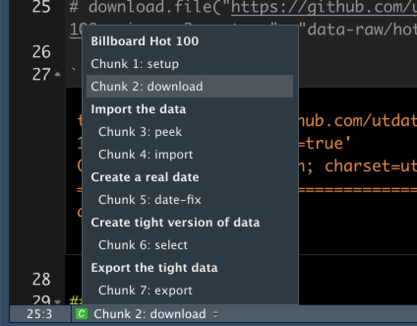
You’ll notice that each Markdown headline you have is listed. My chunks also have names, but yours probably don’t. It’s optional to name chunks with a label but it helps you find them through the bookmarks. In addition, plots produced by the chunks will have useful names that make them easier to reference elsewhere, but that’s later lesson in the semester.

Here is how you can name a chunk by using “execution options”, which can control your code output. (This example shows all of the R code chunk.)

```{r}
#| label: select-rows

hot100_clean |> select(title, performer) |> head()
```

Your chunk labels should be short but evocative and should not contain spaces. Hadley Wickham recommends using dashes - to separate words (instead of underscores _) and avoiding other special characters in chunk labels.

You can read more execution options and chunks in R for Data Science.

3.12 Render and publish

Lastly, I want you to render your notebook so you can see the pretty HTML version.

Click the Render button in the toolbar (or use Cmd-Shift-k).

This should open the HTML version of your page in the Viewer pane. Note there is also a button in that View toolbar that will instead open your site in your web browser.

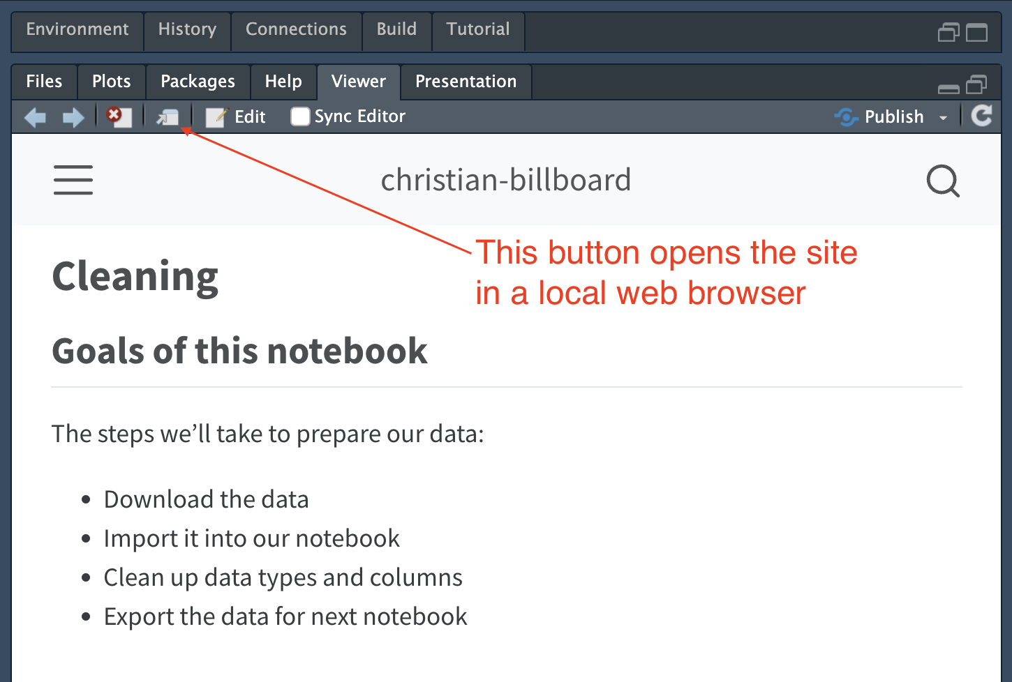
But note this version is only available on your computer. In a minute we’ll publish this to Quarto Pub so you have an online version that we’ll continue to update.

3.12.1 Publish to Quarto pub

Now the we have that in order, let’s publish this to the internet. If you published your last project as instructed, it should remember your credentials.

In the bottom-left pane of RStudio, click on the pane Terminal.
Type in quarto publish.
The first option available (and perhaps the only) should be Quarto Pub. Hit Return to choose that.
It might know who you are already, but continue through the prompts.

You should end up with your browser open to your new Quarto Pub website.

Well done.

3.13 Review of what we’ve learned so far

Most of this lesson has been about importing and cleaning data, which can sometimes be the most challenging part of a project. Here we were working with well-formed data, but we still used quite a few tools from the tidyverse like readr (read_csv, write_rds) and dplyr (select, mutate).

Here are the functions we used and what they do. Most are linked to documentation sites:

library() loads a package so we can use functions within it. We will use at least library(tidyverse) in every project.
read_csv() imports a csv file. You want that function with the underscore, not read.csv.
clean_names() is a function in the janitor package that standardizes column names.
glimpse() is a view of your data where you can see all of the column names, their data type and a few examples of the data.
head() prints the first 6 rows of your data unless you specify differently within the function.
mutate() changes data. You can create new columns or overwrite existing ones.
mdy() is a lubridate function to convert text into a date. There are other functions depending on the way your text is ordered.
select() selects columns from your tibble. You can list all the columns to keep, or use ! to remove columns. There are many variations.
summary() gives you some quick summary statistics about your data like min, max, mean, median.
write_rds() writes data out to a file in a format that preserves data types.

3.14 What’s next

This is part one of a two-chapter project. You might be asked to turn in your progress, or we might wait until both parts are done. Check your class assignments in Canvas.

Please reach out to me if you have questions on what you’ve done so far. These are important skills you’ll use on future projects.