11  Denied Analysis

This is the second of of a two-chapter project. Now that we have assembled and cleaned our data, we need to answer these questions in our followup to the Denied series:

• Has the percentage of special education students in Texas changed since the benchmarking policy was dropped?
• How many districts were above that arbitrary 8.5% benchmark before and after the changes?
• How have local districts changed?

The idea here is to answer those questions through plotting. We’ll use this chapter to walk through the process of using plots to explore and find answers in your data.

11.1 Goals of this chapter

• Introduce datatables() from the DT package
• Practice pivots to prepare data for plotting
• Practice plots to reveal insights in data
• There are wrap-up assignments that include writing, charts and this analysis

When a new concept is introduced, it’s shown and explained here. However, there are also on your own parts where you apply concepts you have learned in previous chapters or assignments.

11.2 Project setup

1. Within the same project you’ve been working, create a new Quarto Notebook. You might call it 02-analysis.qmd.
2. We will be using a new package so you’ll need to install it. Use your Console to run install.packages("DT").
3. Include the libraries below and run them.

library(tidyverse)
library(scales)
library(DT)

11.3 Import cleaned data

1. Create a section for your import
2. Import your cleaned data and call it sped if you want to follow along here.

You should know how to do all that and I don’t know what you called your export file anyway.

But to recap, the data should look like this:

sped |> head()

11.4 Make a searchable table

Wouldn’t it be nice to be able to see the percentage of special education students for each district for each year? The way our data is formatted now, that’s pretty hard to see with our “long” data here.

We could use something more like this? (But with all the years)

distname	cntyname	2013	2014	2015	etc
CAYUGA ISD	ANDERSON	12.3	13.7	13.2	…
ELKHART ISD	ANDERSON	9.1	8.9	10.4	…
FRANKSTON ISD	ANDERSON	10.8	9.7	9.7	…
NECHES ISD	ANDERSON	11.1	9	11.1	…
PALESTINE ISD	ANDERSON	7.7	7.8	8.7	…
WESTWOOD ISD	ANDERSON	9.3	10	9.3	…

And what if you could make that table searchable to find a district by name or county? That would be magic, right?

We can do this by first reshaping our data using pivot_wider() and then applying a function called datatable().

11.4.1 Pivot wider

You used pivot_wider() with the candy data in Chapter 9, so you can look back at how that was done, but here are some hints:

1. Create a new section that notes you are creating a table of district percents.
2. First use select() to get just the columns you need: distname, cntyname, year and sped_percent.
3. Then use pivot_wider()to make a tibble like the one above. Remember that the names_from = argument wants to know which column you want to use to create the names of the new columns. The values_from = argument wants to know which column to pull the cell values from.
4. Save the result into a new tibble and call it district_percents_data

district_percents_data <- sped |> 
  select(distname, cntyname, year, sped_percent) |> 
  pivot_wider(names_from = year, values_from = sped_percent)

11.4.2 Make a datatable

Now comes the magic.

1. In a new R chunk take your district_percents_data and then pipe it into a function called datatable()

district_percents_data |>
  datatable()

That’s kinda brilliant, isn’t it? You know can search by any value in the table.

11.4.3 Data takeaway: How has Austin done

That will be useful tool for you when you are writing about specific districts.

1. Use the data table to find AUSTIN ISD an in your own words, write a data takeaway sentence describing the change over time.

You can see how that might be useful tool for writing about specific districts.

11.5 Choosing a chart to display data

Our first question about this data was this: Has the percentage of special education students in Texas changed since the benchmarking policy was dropped?

Given the data we have, can we answer this?

Let’s think about the charts that might be able to show two related variables like that. Choosing the chart type to display takes experimentation and exploration. Chapter 4 of Nathan Yau’s Data Points book is an excellent look at which chart types help show different data.

This decision tree option might also help you think through it.

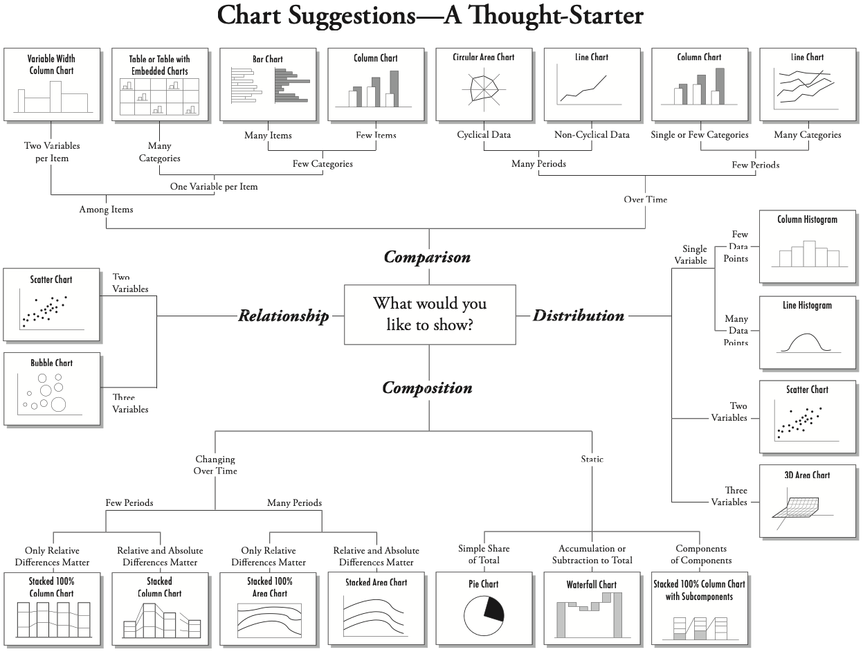
Lastly, another resource to consider this is the ggplot cheatsheet, where it includes possible chart types based on the type of data we are comparing.

11.6 Plot yearly student percentage

I’ll often do a hand drawing of a chart that might help me understand or communicate data. This helps me think about how to summarize and shape my data to get to that point.

For this question Has the percentage of special education students in Texas changed since the benchmarking policy was dropped?, we could show the percentage of special education students for each year. If we are to chart this, the x axis would be the year and the y axis would be the percentage for that year. Perhaps like this:

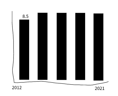
We have the percentage of students in special education for each district in each year. We could get an average of those percentages for each year, but that won’t take into account the size of each district. Some districts have a single-digit number of students while others have hundreds of thousands of students.

But we also have the number of all students in a district with all_count and the number of special education students sped_count. With these, we can build a more accurate percentage across all the districts. This allows us to calculate our student groups by year.

11.6.1 Build the statewide percentage by year data

So, let’s summarize our data. This is a “simple” group_by() and summarize() to get yearly totals, then a mutate() to build our percentage. I’ll supply the logic so you can try writing it yourself.

1. Start a new notebook section and note you are getting yearly percentages
2. In an R chunk, start with your sped data.
3. Group by the year variable.
4. In summarize, create a sum() of the all_count variable. Call this total_students.
5. In the same summarize, create a sum() of the sped_count variable. You might call this total_sped.
6. Check your results at this point … make sure it makes sense.
7. Next use mutate() to create a percentage called sped_percent from your total_students and total_sped summaries. The math for percentage is: (part / whole) * 100. You might want to round that resulting value to tenths as well.
8. I suggest you save all that into a new tibble called yearly_percent (because that’s what I’m gonna do).

yearly_percent <- sped |> 
  group_by(year) |> 
  summarise(
    total_students = sum(all_count),
    total_sped = sum(sped_count)
  ) |> 
  mutate(sped_percent = ((total_sped / total_students) * 100) |> round(1))

yearly_percent

11.6.2 Build the statewide percentage chart

And with that table, you can plot your chart using the year and sped_percent.

1yearly_percent |>
2  ggplot(aes(x = year, y = sped_percent)) +
3  geom_col() +
4  geom_text(aes(label = sped_percent, vjust = -.5))

1

I start with the data AND THEN pipe into ggplot.

2

Within ggplot, set the aesthetics for the x and y axis.

3

Add geom_col() to build the chart. This is better than geom_bar() because it assumes one number and one categorical datum.

4

The geom_text() plots the labels on top of the bars based sped_percent but we need to adjust them with vjust = to move them above the bar.

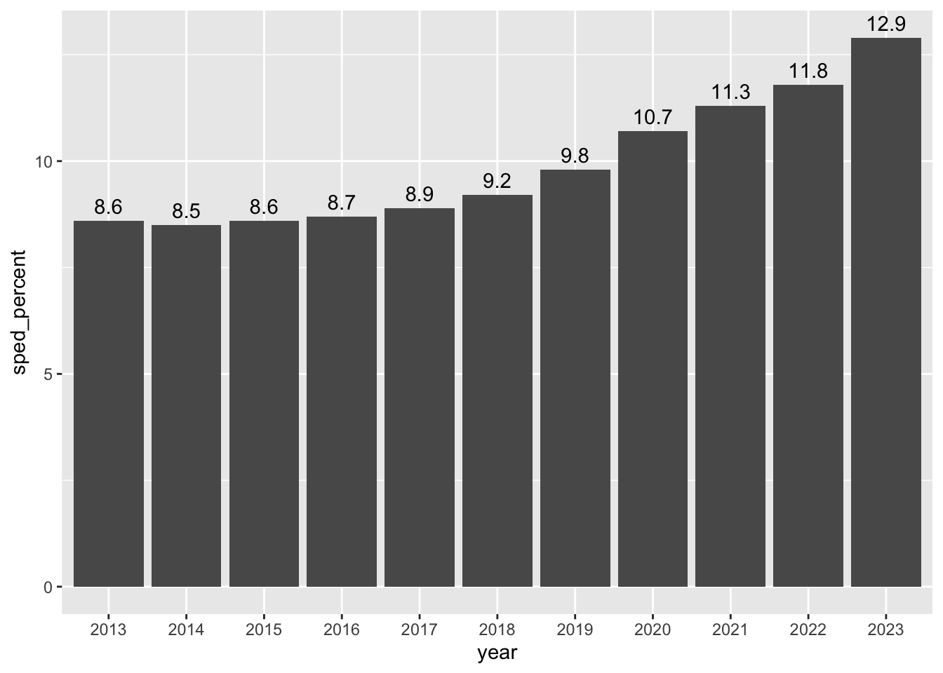
This definitely shows us that the percentage of students in special education (in traditional public schools) has increased each year since 2017 when the benchmark was dropped and then outlawed by the legislature.

I would be careful about saying the increase is because of the changes (though that is likely true), but you can certainly say with authority that it has gone up, and interview other people to pontificate on the reasons why.

BTW, if you wanted to make that chart in datawrapper, you could use the same data structure.

11.6.3 Data takeaway: State percentage

1. Write a data takeaway that describes how the statewide percentage of special education students has changed over time.

The COVID factor

Since we are staring at 2021 and 2022 numbers here, we have an opportunity to discuss how the “COVID era” will have a lasting affect on education data and many other data sources. The adjustments and adaptations that schools had to make changed our world and the data gathered during that time. While our world is always evolving, COVID affected some aspects of our society in profound and lasting ways, and we need to recognize that in our reporting.

In this case, as in many others you will come across in the wild, there isn’t much we can do other than to recognize it was a different time. If the COVID effect is strong enough, we might specifically note it in our charts or stories. In the end, this is the data we have from the TEA and there is no regression or alternative we can use to “normalize” our data to previous times.

11.7 Districts by benchmark and year

Our second question is this: How many districts were above that arbitrary 8.5% benchmark before and after the changes?

It was in anticipation for this that we built the audit_flag field in our data. With that we can count how many rows have the “ABOVE” or “BELOW” value. (In reality, it’s probably at this point we would discover that might be useful that field is and have to go back to the cleaning notebook to create it. I wanted to get that part out of the way so we can concentrate on the charts.)

To decide on which chart to build, we can go back to our chart decision workflow or consult the ggplot cheetsheet. Given we have the discrete values of audit_flag and years, and we want to plot how many districts are counted (which is a continuous value), we’re looking at a stacked or grouped column/bar chart or a line chart.

11.7.1 Summarize the audit flag data

Before we can build the chart, we need to summarize our data. The logic is this: We need to group our data by both the year and the audit_flag, and then count the number of rows for those values.

1. Start a new Markdown section and note you are counting districts by the audit flag.
2. Start with your original sped data.
3. Group your data by both year and audit_flag.
4. Summarize your data by counting n() the results. Name the variable count_districts.
5. Save the resulting data into a tibble called flag_count_districts. You might print that result out so you can refer to it.

flag_count_districts <- sped |> 
  count(year, audit_flag, name = "count_districts")

# I used count()

The data should look like this:

11.7.2 Build the audit flag chart

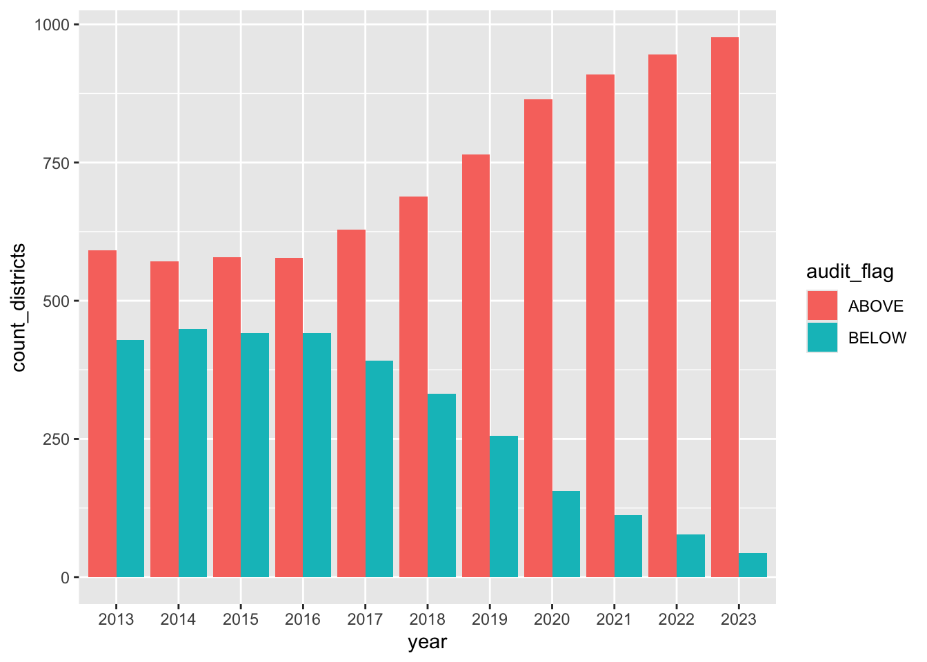
Now that we have the data, we can build the ggplot column chart. The key new thing here is we are using a new aesthetic fill to apply colors based on the audit_flag column.

1. Add some notes you are buliding the first exploratory chart
2. Add an R chunk with the following:

flag_count_districts |> 
  ggplot(aes(x = year, y = count_districts, fill = audit_flag)) +
  geom_col()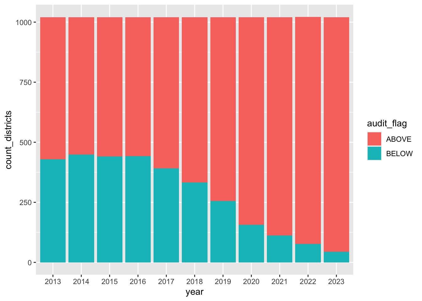

This is actually not a bad look because it does clearly show the number of districts below the 8.5% audit benchmark is dropping year by year, and the number of districts above is growing.

Leave that chart there for reference, but let’s build a new one that is almost the same, but we’ll adjust it to be a grouped column chart instead of stacked. The key difference is we are adding position = "dodge" to the column geom.

1. Note in Markdown text you are building the grouped column version
2. Add a new chunk and start with exactly what you have above.
3. Update the column geom to this: geom_col(position = "dodge")

flag_count_districts |> 
  ggplot(aes(x = year, y = count_districts, fill = audit_flag)) +
1  geom_col(position = "dodge")

1

This is where we add position = "dodge" to set the bars side-by-side.

That’s not bad at all … it might be the winner.

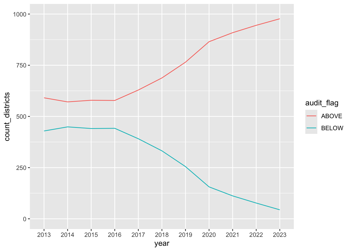
Lastly, let’s chart this data as a line chart to see if that looks any better or is easier to comprehend.

1. Note you are visualizing as a line
2. Add the chunk below.

flag_count_districts |> 
  ggplot(aes(x = year, y = count_districts, group = audit_flag)) +
  geom_line(aes(color = audit_flag)) +
1  ylim(0,1000)

1

We added ylim() here because the default didn’t start the y axis at zero. ylim is used here as a shortcut for scale_y_continuous(limits = c(0,1000)).

11.7.3 Which chart is best?

Remember, this is the question you are trying to answer: How many districts were above that arbitrary 8.5% benchmark before and after the changes?

Both the stacked bar chart and the the grouped bar chart explain this concept. I like the grouped bars a little better because the stacked one kind of looks like all the bars are the same height, evoking 100% or something instead of the number of districts (which don’t change that much.) I’m probably over thinking that, TBH. Sometimes you just gotta make a call.

11.7.4 Data takeaway: District benchmarks

1. Now that you’ve seen the same data in three ways, write a data takeaway the describe what you’ve learned.

11.8 Local districts

We have one last question: How have local districts changed? i.e., what are the percentages for districts in Bastrop, Hays, Travis and Williamson counties? We want to make sure none of these buck the overall trend.

You can certainly use the searchable table we made to get an idea of the number of districts and how the numbers have changed, but you can’t see them there. Searching there does reveal there are too many districts to visualize them all at once. Maybe we can chart one county at a time.

Looking at the chart suggestions workflow, we are doing a comparison over time of many categories … so our trusty line chart is the horse to hitch.

To make that line chart we think about our axes and groups: We need our x axis of year, y axis of the sped_percent and we need to group the lines by their district. Since we need a column that has each year, the long data we started with should suffice:

sped |> head()

We just need to filter that down to a single county cntyname == "BASTROP" to show this. We can even do this all in one code block. Let’s see if you can follow this logic and build Bastrop county for yourself.

1. Start a new section that you are looking at local districts
2. Start a new chunk with your original sped data
3. Filter it to have just rows for BASTROP county
4. Pipe that result into the ggplot() function
5. For the x axis, you are using year, for the y use sped_percent and for group use distname
6. Inside your geom_line() set the the color to the district: aes(color = distname).
7. Do the same for a geom_point() layer.

It should look like this:

sped |> 
  filter(cntyname == "BASTROP") |> 
  ggplot(aes(x = year, y = sped_percent, group = distname)) +
  geom_line(aes(color = distname)) +
  geom_point(aes(color = distname))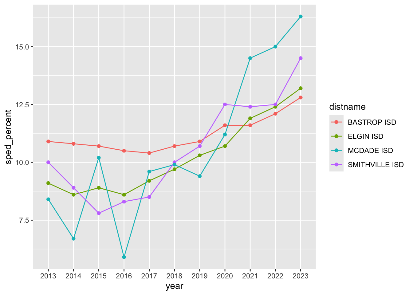

11.8.1 On your own

1. Now do the same for the other three counties, each in their own code chunk: Hays, Travis and Williamson.

These charts give you some reference for the local districts. You’ll see the more districts there are within a county, the less effective the line chart becomes. But at least it gives you an idea of which districts are following the trend.

11.8.2 Data takeaway: The local districts

Write data takeaways about the three counties you’ve looked at.

11.9 Special Education change since 2015

We can see the changes in special education percentages in our chart, but how do we best describe in prose the change from before the law changes (2015) to our current year?

We have two values for each year to work with: The “Count” of special education students in each district, which is the actual number of students in the program; and the “Percentage” of students in special education out of the total in that district

To describe change from one year to the next you might review the Numbers in the Newsroom chapter on Measuring Change (p26). We’ll use Austin ISD numbers from 2015 and 2022 in our examples:

11.9.1 Describing the count changes

• We can show the simple difference (or actual change) in the count of students from one year to the next. There were 8354 students in 2015 and 9396 in 2022:
  • New Count - Old Count = Simple Difference
  • Example: 9396 - 8354 = 1042
  • “Austin ISD served 1,000 more special education students in 2023 (9,396 students) compared to 2015 (8,354 students)”. (I rounded at the beginning for simplicity.)
• We can show the percent change in the count of students from one year to the next:
  • ((New Count - Old Count) / Old Count) * 100 = Percent change
  • Example: ((9396 - 8354) \ 8354) * 100 = 12.5%
  • “The number of special education students served increased 12% from 8,354 in 2015 to 9,396 in 2022.” (Again, I rounded the percent change, but kept the actual counts. The counts could be rounded as well.)

This is accurate, but the percent change can be blown out of proportion when you are dealing with small number. In a small district, moving from 2 to 4 students is a 200% change.

11.9.2 Describing percentage differences

We also have the percentage of special education students in the school, which could be important. This is the share of students that are in the program compared to the total students in the school.

• We can find the percentage point difference from one year to the next using simple difference again, but we have the describe the change as the difference in percentage points:
  • New Percentage - Old Percentage = Percentage Point Difference
  • Example: 13.1% - 9.9% = 3.2 percentage points (NOT 3.2%).
  • “The share of students in special education grew by 3.2 percentage points, from 9.9% in 2015 to 13.1% in 2022.”
• We can find the percent change of share from one year to the next, but we have to again be very specific about what we are talking about … the growth (or decrease) of the share of students in special education.
  • ((New Percentage - Old Percentage) / Old Percentage * 100) = Change in share of students
  • Example: ((13.1 - 9.9) / 9.9) * 100 = 32.3.
  • “The share of students in special education grew by a third from 10% of students in 2015 to 13% of students in 2020.” This describes the growth in the share of students in the program, not the number of special education students overall. I also rounded the percentages.

Describing a “percentage point difference” to readers can be difficult, but perhaps less confusing than describing the “percent change of a percent”.

Great, so which do we use for this story? That depends on what you want to describe. Districts that have fewer special education students to begin with will show a more pronounced percent change with any fluctuation. Then again, a district that has a large percentage of students could be gaining a lot of students with a small percentage change. In the end, we might need to use all of these values to describe different kinds of school districts. We are talking about human beings, so perhaps the counts are important.

11.10 Build your data drop

Like you have with previous projects, update your index.qmd file to add the following:

1. Write a one to two sentence summary about the project as a whole. You can work from descriptions in the book.
2. Write a data-driven news lede based on what you think is the most important takeaway from this analysis.
3. Write a source paragraph that explains the source and range of the data used in the project.
4. Write a series of data takeaway sentences based on what you found.

11.11 Turn in your project

1. Make sure everything runs and Renders properly.
2. Publish your changes to Quarto Pub and include the link to your project in your index notebook so I can bask in your glory.
3. Zip your project folder. (Or export to zip if you are using posit.cloud).
4. Upload to the Canvas assignment.

Important

To be clear, it is your zipped project I am grading. The Quarto Pub link is for convenience.

11.12 New functions used in this chapter

• We used datatable() to build an interactive, searchable table from our data. It’s part of the DT packages.
• I used count() which is a shortcut for grouping and counting rows of data.