library(tidyverse)13 Grouping by dates
Note
This lesson was pulled out of the Billboard project because it was getting really long, but you’ll need this skill when you are working on your mastery assignments.
It is not uncommon in data journalism to count or sum records by year based on a date within your data. Or even by other date parts like month or week. There are some really nifty features within the lubridate package that make this pretty easy.
We’ll run through some of those scenarios here using the Billboard Hot 100 data we used in Chapters 3 & 4. If you want to follow along, you can create a new Quarto Document in your Billboard project. Or you can just use this for reference.
13.1 Setting up
We need to set up our notebook with libraries and data before we can talk specifics. While we are using the lubridate, it is included as part of tidyverse so we do not need to load it separately.
And we need our cleaned Billboard Hot 100 data. We’ll glimpse the rows and check out the date range so we can remember what we have.
hot100 <- read_rds("data-processed/01-hot100.rds")

hot100 |> glimpse()
Rows: 352,300
Columns: 7
$ chart_date <date> 1958-08-04, 1958-08-04, 1958-08-04, 1958-08-04, 1958-08…
$ current_rank <dbl> 1, 2, 3, 4, 5, 6, 7, 8, 9, 10, 11, 12, 13, 14, 15, 16, 1…
$ title <chr> "Poor Little Fool", "Patricia", "Splish Splash", "Hard H…
$ performer <chr> "Ricky Nelson", "Perez Prado And His Orchestra", "Bobby …
$ previous_rank <dbl> NA, NA, NA, NA, NA, NA, NA, NA, NA, NA, NA, NA, NA, NA, …
$ peak_rank <dbl> 1, 2, 3, 4, 5, 6, 7, 8, 9, 10, 11, 12, 13, 14, 15, 16, 1…
$ wks_on_chart <dbl> 1, 1, 1, 1, 1, 1, 1, 1, 1, 1, 1, 1, 1, 1, 1, 1, 1, 1, 1,…hot100$chart_date |> summary() Min. 1st Qu. Median Mean 3rd Qu. Max.
"1958-08-04" "1975-06-21" "1992-05-09" "1992-05-08" "2009-03-28" "2026-02-07" 13.2 Plucking date parts
If you look at the lubridate cheatsheet under “GET AND SET DATE COMPONENTS” you’ll see functions to pluck out parts of a date, like year(). (There is a web version of that cheatsheet, though I like the PDF better.)
If we have a date, like perhaps Taylor Swift’s birthday, we can pluck the year from it.
year("1989-12-13")[1] 198913.3 Grouping by a date part on the fly
Let’s show how this might be useful through an example question:
Which performer has the most appearances on the chart in a given year?
The logic works like this:
- Group all the records by
performerAND the year of thechart_date - Summarize and count the rows
hot100 |>
  group_by(
1    year(chart_date),
    performer
  ) |>
  summarize(appearances = n()) |>
arrange(desc(appearances))- 1
-
This is where we add the year to the group_by, plucking it from the
chart_datewith theyear()function.
It looks like Morgan Wallen had the most appearances in 2023. There is definitely some kinda story here.
Anyway, notice how the year column name is kinda shite? We would not be able to easily reference that variable later, so we should rename that AS we make the group:
hot100 |>
  group_by(
1    yr = year(chart_date),
    performer
  ) |>
  summarize(appearances = n()) |>
arrange(desc(appearances))- 1
-
I added the
yr =part here.
It is a good practice to rename any grouping variable made from a function like that. FWIW, it would’ve worked if I called the new column year, but I named it yr so I’m less likely to confuse it with the function year(). It’s a personal preference what to name the new column.
13.4 Making reusable date parts
If you think you’ll use a date parts more than once, then it makes sense to create new variables and save them. You might make only one or two, but I’ll build on an example to show you several variations.
Here I’m creating a random sample of data with only the chart_date and title columns just so it is easier to see what we are doing. You would normally work with the whole data frame! Here is our sample:
hot100_sample <-
  hot100 |>
  slice_sample(n = 6) |>
  select(chart_date, title)

hot100_sample
ImportantBuilding up this code chunk
If you are following along in your own notebook, please know I’m BUILDING on the code block below, where each new bit below should be edited into your existing chunk.
As we add on more and more variables you might have to scroll the dataframe to see them.
13.4.1 Let’s make a year
Here’s how we do it:
13.4.2 The magical month
We can also pluck out the month of the date, which is pretty useful if you want to measure seasonality within a year, like hot days of summer, etc. The default month() function pulls the month as a number.
hot100_sample |>
  mutate(
    yr = year(chart_date),
1    mo = month(chart_date)
)- 1
- Here we have added a month column, which gives us the number of the month.
But there are some options within month() to give us month NAMES that are ordered as factors instead of alphabetical.
- 1
-
Here we’ve added a variable using the same
month()function, but it adds an argumentlabel = TRUEto make the value a label for the month name instead of the number. - 2
-
And here, again we use
month()with the label argument, but we also add theabbr = FALSEso it gives us the long name instead of the abbreviation.
Note the datatype <ord> under the column mo_label and mo_long. That means this is an “ordered factor” and that when sorted by those labels it will list in MONTH order instead of alphabetical order, which is quite useful.
13.4.3 Floor dates
Sometimes you want to count the number of records within a month and year, like all the songs in January 2000, then February 2000, etc. One way to do that is to create a floor_date, which gives you the “lowest” date within a certain unit like year or month.
Note that the resulting new variables below are real dates, but they have the “lowered” to the first day of the month or year.
- 1
-
The
mo_floorgives you the first day of the month for thatchart_date. - 2
-
The
yr_floorgives you the first day of the year for thatchart_date.
13.5 Saving date parts
Once we know we need these date parts, we can save them into a new data object and use that.
Some things to note with what I’m doing with this code chunk:
- I changed the originating data from our hot100_sample to our actual hot100 data frame.
- I’m also making a “mutate machine” with a glimpse at the end so I can see all the new variables.
- I typically go back to my cleaning notebook to add these once I recognize I need them, and then rerun everything.
hot100_dateparts <-
  hot100 |>
  mutate(
    yr = year(chart_date),
    mo = month(chart_date),
    mo_label = month(chart_date, label = TRUE),
    mo_long = month(chart_date, label = TRUE, abbr = FALSE),
    mo_floor = floor_date(chart_date, unit = "month"),
    yr_floor = floor_date(chart_date, unit = "year")
  )

hot100_dateparts |> glimpse()
Rows: 352,300
Columns: 13
$ chart_date <date> 1958-08-04, 1958-08-04, 1958-08-04, 1958-08-04, 1958-08…
$ current_rank <dbl> 1, 2, 3, 4, 5, 6, 7, 8, 9, 10, 11, 12, 13, 14, 15, 16, 1…
$ title <chr> "Poor Little Fool", "Patricia", "Splish Splash", "Hard H…
$ performer <chr> "Ricky Nelson", "Perez Prado And His Orchestra", "Bobby …
$ previous_rank <dbl> NA, NA, NA, NA, NA, NA, NA, NA, NA, NA, NA, NA, NA, NA, …
$ peak_rank <dbl> 1, 2, 3, 4, 5, 6, 7, 8, 9, 10, 11, 12, 13, 14, 15, 16, 1…
$ wks_on_chart <dbl> 1, 1, 1, 1, 1, 1, 1, 1, 1, 1, 1, 1, 1, 1, 1, 1, 1, 1, 1,…
$ yr <dbl> 1958, 1958, 1958, 1958, 1958, 1958, 1958, 1958, 1958, 19…
$ mo <dbl> 8, 8, 8, 8, 8, 8, 8, 8, 8, 8, 8, 8, 8, 8, 8, 8, 8, 8, 8,…
$ mo_label <ord> Aug, Aug, Aug, Aug, Aug, Aug, Aug, Aug, Aug, Aug, Aug, A…
$ mo_long <ord> August, August, August, August, August, August, August, …
$ mo_floor <date> 1958-08-01, 1958-08-01, 1958-08-01, 1958-08-01, 1958-08…
$ yr_floor <date> 1958-01-01, 1958-01-01, 1958-01-01, 1958-01-01, 1958-01…Now I can use that new hot100_dateparts object with the rest of my analysis.
13.5.1 Use the parts!
Let’s put this to use with an example. I’ll use that mo_floor find Recent appearances by Taylor Swift by month.
swift_month <-
  hot100_dateparts |>
  filter(
    performer == "Taylor Swift",
    chart_date >= "2020-07-01"
  ) |>
  group_by(mo_floor) |>
  summarize(appearances = n())

swift_month
And chart it:
swift_month_plot <-
  swift_month |>
  ggplot(aes(x = mo_floor, y = appearances)) +
  geom_col() +
  geom_text(aes(label = appearances), vjust = -.3) +
  scale_x_date(date_labels="%b %Y", date_breaks  ="1 year", minor_breaks = "1 month") +
  guides(x =  guide_axis(angle = 45)) +
  labs(
    x = "Month and Year",
    y = "Number of appearances",
    title = "Swifts\' \"Midnights\" drives most hits",
    subtitle = str_wrap("While her most recent new album drove the most appearances on the Billboard Hot 100 within a month, each \"Taylor\'s version\"  album since 'Folklore' has also generated hits.")
  )

ggsave("figures/swift_month_plot.png")
Saving 7 x 5 in image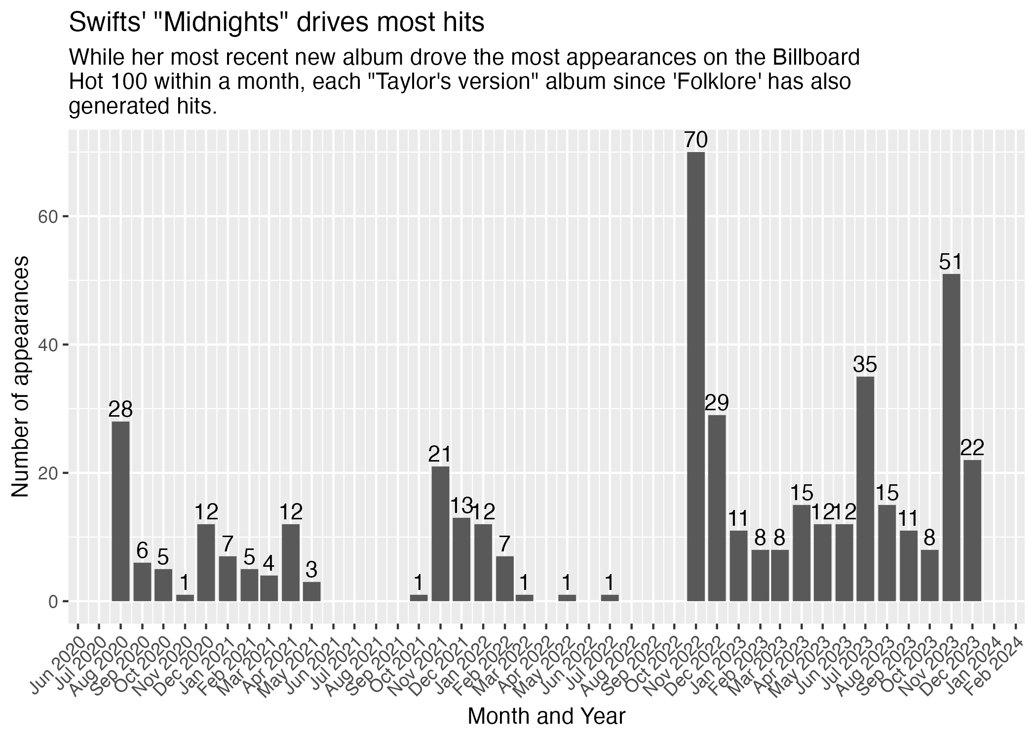
Can you guess when she released her albums?