5 Military Surplus Cleaning

This chapter is by Prof. McDonald, who uses macOS.

Warning

Because of data updates, your answers may differ slightly from what is presented here.

With our Billboard assignment, we went through some common data wrangling processes — importing data, cleaning it and querying it for answers. All of our answers involved using group_by, summmarize and arrange (which I dub GSA) and we summarized with n() to count the number of rows within our groups.

For this data story we need the GSA summary trio again, but we will use math operations within our summarize functions, mainly sum() to add values together.

5.1 About the story: Military surplus transfers

After the 2014 death of Michael Brown and the unrest that followed, there was widespread criticism of Ferguson, Mo. police officers for their use of military-grade weapons and vehicles. There was also heightened scrutiny to a federal program that transfers unused military equipment to local law enforcement. Many news outlets, including NPR and Buzzfeed News, did stories based on data from the “1033 program” handled through the Law Enforcement Support Office. Buzzfeed News also did a followup report in 2020 where reporter John Templon published his data analysis, which he did using Python.

You will analyze the same dataset to see how Central Texas police agencies have used the program and write a short data drop about transfers to those agencies.

5.1.1 The 1033 program

To work through this story we need to understand how this transfer program works. You can read all about it here, but here is the gist:

In 1997, Congress approved the “1033 program” that allows the U.S. military to give “surplus” equipment that they no longer need to law enforcement agencies like city police forces. The program is run by the Law Enforcement Support Office, which is part of the Defense Logistics Agency (which handles the global defense supply chain for all the branches of the military) within the Department of Defense. (The program is run by the office inside the agency that is part of the department.)

All kinds of equipment moves between the military and these agencies, from boots and water bottles to assault rifles and cargo planes. The local agency only pays for shipping the equipment, but that shipping cost isn’t listed in the data. What is in the data is the “original value” of the equipment in dollars, but we can’t say the agency paid for it, because they didn’t.

Property falls into two categories: controlled and non-controlled. Controlled property “consists of military items that are provided via a conditional transfer or ‘loan’ basis where title remains with DoD/DLA. This includes items such as small arms/personal weapons, demilitarized vehicles and aircraft and night vision equipment. This property always remains in the LESO property book because it still belongs to and is accountable to the Department of Defense. When a local law enforcement agency no longer wants the controlled property, it must be returned to Law Enforcement Support Office for proper disposition.” This is explained in the LESO FAQ.

But most of the transfers to local agencies are for non-controlled property that can be sold to the general public, like boots and blankets. Those items are removed from the data after one year, unless it is deemed a special circumstance.

The agency releases data quarterly, but it is really a “snapshot in time” and not a complete history. Those non-controlled items transferred more than a year prior are missing, as are any controlled items returned to the feds.

5.1.2 About the data

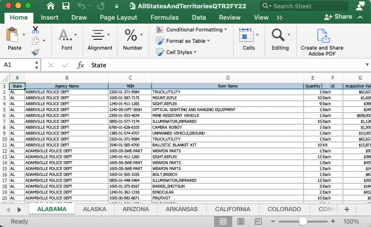
The data comes in a spreadsheet that has a different tab for each state and territory. I’ve done some initial work on the original data that is beyond the scope of this class, so we’ll use my copy of the data. I will supply a link to the combined data below.

There is no data dictionary or record layout included with the data but I have corresponded with the Defense Logistics Agency to get a decent understanding of what is included.

sheet: Which sheet the data came from. This is an artifact from the data merging script.
state: A two-letter designation for the state of the agency.
agency_name: This is the agency that got the equipment.
nsn: The National Stock Number, a special ID that identifies the item in a government supplies database.
item_name: The item transferred. Googling the names can sometimes yield more info on specific items, or you can search by nsn for more info.
quantity: The number of the “units” the agency received.
ui: Unit of measurement (item, kit, etc.)
acquisition_value: a cost per unit for the item.
demil_code: Categories (as single letter key values) that indicate how the item should be disposed of. Full details here.
demil_ic: Also part of the disposal categorization.
ship_date: The date the item(s) were sent to the agency.
station_type: What kind of law enforcement agency made the request.

Here is a glimpse of a sample of the data:

Rows: 10
Columns: 12
$ sheet             <dbl> 17, 42, 5, 45, 36, 33, 5, 22, 3, 22
$ state             <chr> "KY", "SC", "CA", "TX", "OH", "NC", "CA", "MI", "AZ"…
$ agency_name       <chr> "MEADE COUNTY SHERIFF DEPT", "PROSPERITY POLICE DEPT…
$ nsn               <chr> "6115-01-435-1567", "1005-00-589-1271", "7520-01-519…
$ item_name         <chr> "GENERATOR SET,DIESEL ENGINE", "RIFLE,7.62 MILLIMETE…
$ quantity          <dbl> 5, 1, 32, 1, 1, 1, 1, 1, 1, 1
$ ui                <chr> "Each", "Each", "Dozen", "Each", "Each", "Each", "Ea…
$ acquisition_value <dbl> 4623.09, 138.00, 16.91, 749.00, 749.00, 138.00, 499.…
$ demil_code        <chr> "A", "D", "A", "D", "D", "D", "D", "D", "D", "D"
$ demil_ic          <dbl> 1, 1, 1, 1, 1, 1, 1, 1, 1, 1
$ ship_date         <dttm> 2021-03-22, 2007-08-07, 2020-10-29, 2014-11-18, 2014…
$ station_type      <chr> "State", "State", "State", "State", "State", "State"…

And a look at just some of the more important columns:

leso_sample |> 
  select(agency_name, item_name, quantity, acquisition_value)

Each row of data is a transfer of a particular type of item from the U.S. Department of Defense to a local law enforcement agency. The row includes the name of the item, the quantity, and the value ($) of a single unit.

What the data doesn’t have is the total value of the items in the shipment. If there are 5 generators as noted in the first row above and the cost of each one is $4623.09, we have to multiply the quantity times the acquisition_value to get the total value of that equipment.

The data also doesn’t have any variable indicating if an item is controlled or non-controlled, but I’ve corresponded with the Defense Logistics Agency to gain a pretty good understanding of how to isolate them based on the demilitarization codes.

These are things I learned about by talking to the agency and reading through documentation. This kind of reporting and understanding ABOUT your data is vital to avoid mistakes.

5.2 The questions we will answer

All answers should be based on controlled items given to Texas agencies from Jan. 1, 2010 to present.

How many total “controlled” items were transferred to Texas agencies, and what are they all worth? We’ll summarize all the controlled items only to get the total quantity and total value of everything.
How many total “controlled” items did each agency get and how much was it all worth? Which agency got the most stuff?
- How about local police agencies? I’ll give you a list.
What specific “controlled” items did each agency get and how much were they worth? Now we’re looking at the kinds of items.
- What did local agencies get?

You’ll research some of the more interesting items the agencies received so you can include them in a short data drop.

5.3 Getting started: Create your project

Note

If you are using posit.cloud, you’ll want to refer to the Using posit.cloud chapter to create your project, using the material below as necessary.

We will build the same project structure that we did with the Billboard project. In fact, all our class projects will have this structure. Since we’ve done this before, some of the directions are less detailed.

With RStudio open, make sure you don’t have a project open. Go to File > Close project.
Use the create project button (or File > New project) to create a new project in a New Directory.
For the project type, choose Quarto Website
Name the directory “yourname-military-surplus”, but with your name.
Create two folders: data-raw and data-processed.
In the index.qmd file, replace the title value with “Military Surplus”, as that is our project title.
Remove the boilerplate stuff after the YAML title and this bit about the project:

This project looks at how much U.S. military surplus equipment has been transferred to law enforcement agencies. It uses data from from the "1033 program" handled through the [Law Enforcement Support Office](https://www.dla.mil/Disposition-Services/Offers/Law-Enforcement/Public-Information/), which posts data quarterly.

You’ll come back to this at the end of the project to write your summary.

5.4 Cleaning notebook

Again, like Billboard, we’ll create a notebook specifically for downloading, cleaning and prepping our data.

Create a new Quarto Document.
For the title use “Cleaning”.
Remove the rest of the boilerplate template.
Save the file and name it 01-cleaning.qmd.
Open _quarto.yml and change the navigation link from about.qmd to 01-cleaning.qmd.

5.4.1 The goals of the notebook

As noted before, I separate cleaning into a separate notebook so that each subsequent analysis notebook can take advantage of that work. It’s the DRY principal in programming: Don’t Repeat Yourself. Often I will be in an analysis notebook realizing that I have more cleaning to do, so I’ll go back to the cleaning notebook, add it and rerun everything. Because I’ve worked with and researched this data, I’m aware of cleaning steps that a newcomer to the data might not be aware of at this point. To save you that time and heartache, we will take advantage of my experience and do all this cleaning work up front even though you haven’t seen the “need” for it yet.

That’s a long-winded opening to say let’s add our notebook goals so you know what’s going on here.

In Markdown, add a headline noting these are notebook goals.
Add the goals below as text:

- Download the data
- Import the data
- Check datatypes
- Create a total_value variable
- Create a control_type variable
- Filter the date range (since Jan. 1 2010)
- Export the cleaned data

5.4.2 Add a setup section

This is the section in the notebook where we add our libraries and such. Again, every notebook has this section, though the packages used may vary on need. This time (and each time hense) we will add some “execution options” to our setup chunk.

Add a headline called “Setup” and text about what we are doing, adding our libraries.
Add your setup code chunk with the code below.

```{r}
#| label: setup
#| message: false

library(tidyverse)
```

Some reminders:

The #| label: setup is special in that it will be run first no matter where we are in the notebook. Helpful to make sure your libraries are loaded.
The #| message: false option silences the message about all the different packages in the tidyverse when the library is loaded. It just cleans up the notebook.

One other note about this … we should only need the tidyverse library for this notebook because the data already has clean names (no need for janitor.)

5.5 Download the data

A new section means a new headline and description. Add it. It is good practice to describe and link to the data you will be using. You can use the text below:

While the data we will use here if from Prof. McDonald, it is from the [Law Enforcement Support Office](https://www.dla.mil/DispositionServices/Offers/Reutilization/LawEnforcement/PublicInformation/). Find more information [about the program here](https://www.dla.mil/DispositionServices/Offers/Reutilization/LawEnforcement/ProgramFAQs/).

Tip

Note the text above scrolls off the screen. Use the copy icon to select all the text.

Use the download.file() function to download the date into your data-raw folder. Remember you need two arguments:

download.file(
  "url_to_data",
  "path_to_folder/filename.csv",
  mode = "wb"
)

What you need:

The data can be found at this url below
It should be saved into your data-raw folder with a name for the file.

https://github.com/utdata/rwd-r-leso/blob/main/data-processed/leso.csv?raw=true

Try writing this on your own

# You can comment the lines below once you have the data
download.file(
  "https://github.com/utdata/rwd-r-leso/blob/main/data-processed/leso.csv?raw=true",
  "data-raw/leso.csv",
  mode = "wb"
)

Once you’ve built your code chunk and run it, you should make sure the file downloaded into the correct place: in your data-raw folder.

Tip

If you get an error about the path, you might make sure you created the data-raw folder first.

5.6 Import the data

It’s time to import the data into the notebook. Like the Billboard project, we are again working with a CSV, or comma-separated-values text file.

Add a new Markdown section noting you are doing the import. Include a headline, text and a new code chunk.

I suggest you build the code chunk a bit at a time in this order:

Use read_csv() to read the file from our data-raw folder.
Edit that line to put the result into a tibble object using <-. Name your new tibble leso.
Print the tibble as a table to the screen again by putting the tibble object on a new line and running it. This allows you to see it in columnar form.

Try real hard first before clicking here for the answer.

# assigning the tibble
leso <- read_csv("data-raw/leso.csv")
# printing the tibble
leso

The output you get will be the table, which looks sort of like this, but I’m just showing the first six lines:

5.6.1 Glimpse the data

In a new code block, print the tibble but pipe it into glimpse() so you can see all the column names.

leso |>  glimpse()

Rows: 99,052
Columns: 12
$ sheet             <dbl> 1, 1, 1, 1, 1, 1, 1, 1, 1, 1, 1, 1, 1, 1, 1, 1, 1, 1…
$ state             <chr> "AL", "AL", "AL", "AL", "AL", "AL", "AL", "AL", "AL"…
$ agency_name       <chr> "ABBEVILLE POLICE DEPT", "ABBEVILLE POLICE DEPT", "A…
$ nsn               <chr> "1005-01-587-7175", "1240-01-411-1265", "2320-01-371…
$ item_name         <chr> "MOUNT,RIFLE", "SIGHT,REFLEX", "TRUCK,UTILITY", "BAL…
$ quantity          <dbl> 10, 9, 1, 10, 1, 1, 1, 3, 1, 1, 1, 1, 1, 1, 1, 1, 1,…
$ ui                <chr> "Each", "Each", "Each", "Kit", "Each", "Each", "Each…
$ acquisition_value <dbl> 1626.00, 371.00, 62627.00, 17264.71, 62627.00, 65800…
$ demil_code        <chr> "D", "D", "C", "D", "C", "C", "Q", "D", "C", "D", "D…
$ demil_ic          <dbl> 1, 1, 1, 1, 1, 1, 3, 1, 1, 1, 1, 1, 1, 1, 1, 1, 1, 1…
$ ship_date         <dttm> 2016-09-19, 2016-09-14, 2016-09-29, 2018-01-30, 201…
$ station_type      <chr> "State", "State", "State", "State", "State", "State"…

5.7 Checking datatypes

Take a look at your glimpse returns. These are the things to watch for:

Are your variable names (column names) clean? All lowercase with _ separating words?
Are dates saved in a date format? ship_date looks good at <dttm>, which means “datetime”.
Are your numbers really numbers? acquisition_value is the column we are most concerned about here, and it looks good.

This data set looks good (because I pre-prepared it for you), but you always want to check and make corrections, like we did to fix the date in the Billboard assignment.

5.8 Remove unnecessary columns

Sometimes at this point in a project, you might not know what columns you need to keep and which you could do without. The nice thing about doing this with code in a notebook is we can always go back, make corrections and run our notebook again. In this case, we will remove the sheet variable since we don’t need it. (It’s an artifact of the processing I’ve done on the file.)

Start a new section with a headline and text to explain you are removing unneeded columns.
Add a code chunk and the following code. I’ll explain it below.

1leso_tight <- leso |>
2  select(!sheet)

3leso_tight |> glimpse()

1: We create a new tibble leso_tight and then fill it with leso data AND THEN …
2: We use select to remove the column called sheet. Within the select() function, we use ! to “negate” the column called “sheet”.
3: We then glimpse the new data.

Rows: 99,052
Columns: 11
$ state             <chr> "AL", "AL", "AL", "AL", "AL", "AL", "AL", "AL", "AL"…
$ agency_name       <chr> "ABBEVILLE POLICE DEPT", "ABBEVILLE POLICE DEPT", "A…
$ nsn               <chr> "1005-01-587-7175", "1240-01-411-1265", "2320-01-371…
$ item_name         <chr> "MOUNT,RIFLE", "SIGHT,REFLEX", "TRUCK,UTILITY", "BAL…
$ quantity          <dbl> 10, 9, 1, 10, 1, 1, 1, 3, 1, 1, 1, 1, 1, 1, 1, 1, 1,…
$ ui                <chr> "Each", "Each", "Each", "Kit", "Each", "Each", "Each…
$ acquisition_value <dbl> 1626.00, 371.00, 62627.00, 17264.71, 62627.00, 65800…
$ demil_code        <chr> "D", "D", "C", "D", "C", "C", "Q", "D", "C", "D", "D…
$ demil_ic          <dbl> 1, 1, 1, 1, 1, 1, 3, 1, 1, 1, 1, 1, 1, 1, 1, 1, 1, 1…
$ ship_date         <dttm> 2016-09-19, 2016-09-14, 2016-09-29, 2018-01-30, 201…
$ station_type      <chr> "State", "State", "State", "State", "State", "State"…

If we wanted to remove more than one column — say both sheet and station_type — then we would use ! negate in conjunction with the c() function to combine items into a new vector, like this: select(!c(sheet, station_type)). The use of ! to remove things will come up in other places in R, as will using c() to combine things together.

So now we have a tibble called leso_tight that we will work with in the next section.

5.9 Create a total_value column

During my reporting about this data I learned that the acquisition_value noted in the data is for a single “unit” of each item. If the shipment item was a rifle with a quantity of “5” and acquisition_value of “200”, then each rifle is worth $200, but the total shipment would be 5 times $200, or $1,000. That $1000 total value is not listed in the data, so we need to add it.

Let’s walk through how to do that with a different example.

When we used mutate() to convert the date in the Billboard assignment, we were reassigning values in each row of a column back into the same column.

In this assignment, we will use mutate() to create a new column with new values based on a calculation. Let’s review the concept first.

If you started with data like this:

item	item_count	item_value
Bread	2	1.5
Milk	1	2.75
Beer	3	9

And then wanted to create a total value of each item in the table, you would use mutate():

# Don't put this in your notebook. It's just explanation.
data |> 
  mutate(total_value = item_count * item_value)

You would get a return like this, with your new total_value column added at the end:

item	item_count	item_value	total_value
Bread	2	1.5	3
Milk	1	2.75	2.75
Beer	3	9	27

Other math operators work as well: +, -, * and /.

So, now that we’ve talked about how it is done, I want you to:

Create a new section with headline, text and code chunk.
Use mutate() to create a new total_value column that multiplies quantity times acquisition_value.
Assign those results into a new tibble called leso_total so we can all be on the same page.
Glimpse the new tibble so you can check the results.

Try it on your own. You can figure it out!

leso_total <- leso_tight |> 
  mutate(
    total_value = quantity * acquisition_value
  )

leso_total |> glimpse()

Rows: 99,052
Columns: 12
$ state             <chr> "AL", "AL", "AL", "AL", "AL", "AL", "AL", "AL", "AL"…
$ agency_name       <chr> "ABBEVILLE POLICE DEPT", "ABBEVILLE POLICE DEPT", "A…
$ nsn               <chr> "1005-01-587-7175", "1240-01-411-1265", "2320-01-371…
$ item_name         <chr> "MOUNT,RIFLE", "SIGHT,REFLEX", "TRUCK,UTILITY", "BAL…
$ quantity          <dbl> 10, 9, 1, 10, 1, 1, 1, 3, 1, 1, 1, 1, 1, 1, 1, 1, 1,…
$ ui                <chr> "Each", "Each", "Each", "Kit", "Each", "Each", "Each…
$ acquisition_value <dbl> 1626.00, 371.00, 62627.00, 17264.71, 62627.00, 65800…
$ demil_code        <chr> "D", "D", "C", "D", "C", "C", "Q", "D", "C", "D", "D…
$ demil_ic          <dbl> 1, 1, 1, 1, 1, 1, 3, 1, 1, 1, 1, 1, 1, 1, 1, 1, 1, 1…
$ ship_date         <dttm> 2016-09-19, 2016-09-14, 2016-09-29, 2018-01-30, 201…
$ station_type      <chr> "State", "State", "State", "State", "State", "State"…
$ total_value       <dbl> 16260.0, 3339.0, 62627.0, 172647.1, 62627.0, 658000.…

5.9.1 Check that it worked!!

Note that new columns are added at the end of the tibble. Sometimes you can look through the glimpsed data to see if your mutate worked correctly, but that depends on the data.

If there isn’t enough information visible, you can print some sample rows of the data to peek through it.

Add some text that you are checking the results.
Add a new chunk and pipe leso_total into a new function slice_sample(n = 10).

leso_total |>
1  slice_sample(n = 10)

1: The argument n = 10 is the number of rows to show. The default is a single row.

At this point you can page through the columns to check the math. If you want to see a different sample of data, just rerun the chunk as you get a new one each time. If you want a different number of lines, change the value inside the function.

But even with this, there are a lot of columns to page through. You can use add on select() to pluck out the columns of interest to check.

Edit your chunk’s last line like this:

leso_total |> 
  slice_sample(n = 10) |>
  select(agency_name, quantity, acquisition_value, total_value)

This should allow you to check if the math worked. In one of my samples there was a record for “JONESBORO POLICE DEPARTMENT” that has a quantity of “6” and acquisition_value of “114.00” and I got a total_value of “684.00”. So, 6 * 114.00 = 684.00, which is correct!

Something to note about this process: In the first part of this chunk we are taking leso_tight, making some changes to it and the saving it into leso_total. We have two objects now, one before the changes and one after.

In the last part of the chunk, we are taking leso_total object and we are peeking at some rows and some columns, but we are not saving those changes into a new object. There is no <- operator here. We are just printing the results to the screen so we can see parts of the data more clearly.

5.10 Controlled vs. non-controlled

Again, by reading through the documentation about this data I learned about controlled vs non-controlled property. Basically non-controlled generic items like boots and blankets are removed from the data after one year, but controlled items like guns and airplanes remain on the list until they are returned to the military for disposal. We are only concerned with the controlled items.

There isn’t anything within the data that says it is “controlled” and really no clear indication in the documentation on how to tell what is what. So, I emailed the agency and asked them. Here is an edited version of their answer:

Property with the DEMIL codes A and Q6 are considered non-controlled general property and fall off the LESO property books after one year. All other Demil codes are considered controlled items and stay on the LESO property book until returned to DLA for disposition/disposal. However, there are some exceptions. For instance, aircraft are always controlled regardless of the demil code. Also, LESO has the discretion to keep items as controlled despite the demil code. This happens with some high value items. There isn’t a standard minimum value. It also may also depend on the type of property.

This actually took some back and forth to figure out, as I had noticed there were AIRPLANE, CARGO-TRANSPORT items in the data that were older than a year, along with some surveillance robots. That’s when they replied about the airplanes, but it turns out the robots were simply an error. Data is dirty when humans get involved; somebody coded it wrong.

These “DEMIL codes” they referenced are the demil_code and demil_ic columns in the data, so we can use those to mark which records are “non-controlled” (A and Q6) and then mark all the rest as “controlled”. We know of one exception – airplanes – which we need to mark controlled. We can’t do much with the “high value” items since there isn’t a specific maximum value to test. We’ll just have to note that in our story, something like “the agency has discretion to designate as as controlled, such as high value items, but they are not categorized as such and may have been dropped from our analysis.”

But, we can catch most of them … we just need to work through the logic. This is not an uncommon challenge in data science, so we have some tools to do this. Our workhorse here is the case_when() function, where we can make decisions based on values in our data.

In the interest of time and getting this done, I will just provide the code.

leso_control <- leso_total |> 
  mutate(
    control_type = case_when(
      str_detect(item_name, "AIRPLANE") ~ TRUE,
      (demil_code == "A" | (demil_code == "Q" & demil_ic == 6)) ~ FALSE,
      TRUE ~ TRUE
    )
  )

leso_control |> glimpse()

Rows: 99,052
Columns: 13
$ state             <chr> "AL", "AL", "AL", "AL", "AL", "AL", "AL", "AL", "AL"…
$ agency_name       <chr> "ABBEVILLE POLICE DEPT", "ABBEVILLE POLICE DEPT", "A…
$ nsn               <chr> "1005-01-587-7175", "1240-01-411-1265", "2320-01-371…
$ item_name         <chr> "MOUNT,RIFLE", "SIGHT,REFLEX", "TRUCK,UTILITY", "BAL…
$ quantity          <dbl> 10, 9, 1, 10, 1, 1, 1, 3, 1, 1, 1, 1, 1, 1, 1, 1, 1,…
$ ui                <chr> "Each", "Each", "Each", "Kit", "Each", "Each", "Each…
$ acquisition_value <dbl> 1626.00, 371.00, 62627.00, 17264.71, 62627.00, 65800…
$ demil_code        <chr> "D", "D", "C", "D", "C", "C", "Q", "D", "C", "D", "D…
$ demil_ic          <dbl> 1, 1, 1, 1, 1, 1, 3, 1, 1, 1, 1, 1, 1, 1, 1, 1, 1, 1…
$ ship_date         <dttm> 2016-09-19, 2016-09-14, 2016-09-29, 2018-01-30, 201…
$ station_type      <chr> "State", "State", "State", "State", "State", "State"…
$ total_value       <dbl> 16260.0, 3339.0, 62627.0, 172647.1, 62627.0, 658000.…
$ control_type      <lgl> TRUE, TRUE, TRUE, TRUE, TRUE, TRUE, TRUE, TRUE, TRUE…

If you want to learn more about the code in that block, read the Appendix chapter titled Using case_when.

5.11 Filtering our data

In the Billboard lesson you used filter() to get No. 1 songs and to get a date range of data. We need to do something similar here to get only data of a certain date range. We’ll build the filters one at a time so we can save the resulting objects separately.

Create a new section with headlines and text that denote you are filtering the data to records since Jan. 1, 2010.
Create a chunk and filter your leso_control data to get rows with a ship_date later than 2010-01-01.
Save the result into a new tibble called leso_dated.
Print out the new tibble leso_dated.

Write it yourself, but here is the code

leso_dated <- leso_control |> 
  filter(
    ship_date >= "2010-01-01"
  )

leso_dated

5.11.1 Checking the results with summary()

How do you know this date filter worked? Well, my data went from 99052 to 67852 rows, so we did something. You might look at the results table and click over to the ship_date columns so you can see some of the results, but you can’t be sure the top row is the oldest. We could use an arrange() to test that, but I have another suggestion: summary().

Now, summary() is different than summarize(), which we’ll do plenty of in a minute. The summary() function will show you some results about each column in your data, and when it is a number or date, it will give you some basic stats like min, max and median values.

Edit your chunk to not just print out the tibble, but pipe that into summary(), like this:

leso_dated |> summary()

    state           agency_name            nsn             item_name        
 Length:67852       Length:67852       Length:67852       Length:67852      
 Class :character   Class :character   Class :character   Class :character  
 Mode  :character   Mode  :character   Mode  :character   Mode  :character  
                                                                            
                                                                            
                                                                            
                                                                            
    quantity             ui            acquisition_value   demil_code       
 Min.   :    0.00   Length:67852       Min.   :       0   Length:67852      
 1st Qu.:    1.00   Class :character   1st Qu.:     200   Class :character  
 Median :    1.00   Mode  :character   Median :     499   Mode  :character  
 Mean   :    5.66                      Mean   :   22002                     
 3rd Qu.:    1.00                      3rd Qu.:    3578                     
 Max.   :44000.00                      Max.   :22000000                     
                                                                            
    demil_ic       ship_date                      station_type      
 Min.   :0.000   Min.   :2010-01-05 00:00:00.00   Length:67852      
 1st Qu.:1.000   1st Qu.:2012-03-07 00:00:00.00   Class :character  
 Median :1.000   Median :2014-08-27 00:00:00.00   Mode  :character  
 Mean   :1.436   Mean   :2015-08-15 23:52:06.43                     
 3rd Qu.:1.000   3rd Qu.:2018-05-04 00:00:00.00                     
 Max.   :7.000   Max.   :2023-09-29 07:00:14.00                     
 NA's   :5880                                                       
  total_value       control_type   
 Min.   :       0   Mode :logical  
 1st Qu.:     371   FALSE:7918     
 Median :     749   TRUE :59934    
 Mean   :   24066                  
 3rd Qu.:    6392                  
 Max.   :22000000

You should be be able to look at the Min value of ship_date in the summary to make sure there are not dates before 2010. You can also look at the Max value to see your latest ship_date. You should make a mental (and perhaps written) note about that max date.

We now have an object, leso_dated that has all the data since 2010. We’ll export this for our next notebook.

5.12 Export cleaned data

Now that we have our data selected, mutated and filtered how we want it, we can export into .rds files to use in other notebooks. As you may recall from Billboard, we use the .rds format because it will remember data types and such.

Create a new section with headline and text explaining that you are exporting the data.
Do it.

The function you need is called write_rds and you need to give it a path/name that saves the file in the data-processed folder. Name the file with 01- at the beginning so you know it came from the first notebook, and then use a short and descriptive name for the rest. No spaces. Well-formatted, descriptive file names are important to your future self and other colleagues.

Here is my version:

The last chunk. You can do it.

leso_dated |> write_rds("data-processed/01-leso-all.rds")

5.13 Render and clean up your notebook

You should Render your notebook and read it over carefully. Some things to look for:

Make sure you have nice headlines for each of your sections.
Make sure your navigation works for the Home and Cleaning pages.
Flesh out your index.qmd file to make sure the basic assignment information is there.

5.14 Things we learned in this lesson

This chapter was similar to when we imported data for Billboard, but we did introduce a couple of new concepts:

slice_sample(n = 10) gives us 10 random rows from our data.
case_when() allows you to categorize a new column based on logic within your data. There is more about this in the this appendix.
summary() gives you descriptive statistics about your tibble. We used it to check the “min” and “max” date, but you can also see averages (mean) and medians.