10 Denied Cleaning

This is the first of a two-chapter project. It is by Prof. McDonald, using macOS.

So far all of our lessons have come from a single data source, but that’s not always the case in the real world. With this lesson we’ll learn how to import multiple files at once and “bind” them, and to use “join” to enhance that data from a lookup table.

10.1 Goals of the chapter

Import multiple files at once and bind them with map()
Join data frames with inner_join()
Use str_remove() to clean data
Introduce if_else() for categorization

We’ll use the results of this chapter in our next one.

10.2 About the story: Denied

In 2016, the Houston Chronicle published a multi-part series called Denied that outlined how a Texas Education Agency policy started in 2004 could force an audit of schools that have more than 8.5% of their students in special education programs. The story was a Pulitzer Prize finalist. Here’s an excerpt:

Over a decade ago, the officials arbitrarily decided what percentage of students should get special education services — 8.5% — and since then they have forced school districts to comply by strictly auditing those serving too many kids.

Their efforts, which started in 2004 but have never been publicly announced or explained, have saved the Texas Education Agency billions of dollars but denied vital supports to children with autism, attention deficit hyperactivity disorder, dyslexia, epilepsy, mental illnesses, speech impediments, traumatic brain injuries, even blindness and deafness, a Houston Chronicle investigation has found.

More than a dozen teachers and administrators from across the state told the Chronicle they have delayed or denied special education to disabled students in order to stay below the 8.5 percent benchmark. They revealed a variety of methods, from putting kids into a cheaper alternative program known as “Section 504” to persuading parents to pull their children out of public school altogether.

Following the Chronicle’s reporting (along with other news orgs), the Texas Legislature in 2017 unanimously banned using a target or benchmark on how many students a district or charter school enrolls in special education.

We want to look into the result of this reporting based on three things:

Has the percentage of special education students in Texas changed since the benchmarking policy was dropped?
How many districts were above that arbitrary 8.5% benchmark before and after the changes?
How have local districts changed?

To prepare for this:

Read Part 1 of the original Denied series, at least to the heading “A special child.” Pay attention to parts about the “Performance-Based Monitoring Analysis System.”
Read About this series
Read this followup about the legislative changes.

10.3 About the data

Each year, the Texas Education Agency publishes the percentage of students in special education as part of their Texas Academic Performance Reports. We can download a file that has the percentages for each district in the state.

There are some challenges, though:

We have to download each year individually. There are nine years of data.
The are no district names in the files, only a district ID. We can get a reference file, though.
There are some differences in formatting for some files.

I will save you the hassle of going through the TAPR database to find and download the individual files by providing a starter project.

10.3.1 Set up your project

With this project you’ll start with a copy I have prepared for you. How you do that differs a little depending on the RStudio platform you are using.

10.3.1.1 If you are using RStudio Desktop

You will download a project that is already set up for you and then open it.

Use the link below to download the project.

Download rwdir-sped-template-main.zip

Find that file on your computer and uncompress it.
Rename the project folder to yourname-sped but use your name.
Move the project folder to your rwd folder or wherever you’ve been saving your class projects.
In RStudio, choose File > New Project. Choose EXISTING Directory at the next step and then find the folder you saved. Use that to create your project.

10.3.1.2 If you are a posit.cloud user

From your posit.cloud account, go to this shared project
Click Save a permanent copy so you have your own version.
Rename the project yourname-sped but use your name.

10.4 The DSTUD data

To track how percentages of special education students have changed over time, we will use data observations from the Texas Education Agency’s Texas Academic Performance Reports. The TEA has a portal where you can downloaded bulk data by district or campus for each academic year.

While our downloaded starter project has all the data we need, you should go through this process for one of the years just so you see how it works.

The process goes like this:

Start at the Texas Academic Performance Reports page
Choose the school year of interest (choose 2012-13 to just look at the process)
Find the Data Download page
Choose the TAPR Data in Excel (Rates Only) option
Click on District Download. Click Continue to move on.
Choose the Student Information data set and choose Continue.
- Choose the Comma-Delimited (csv) format
- Choose Student: Counts/Percents ¹
- Also choose Student Enrollment by Program ²
- Click Download.

This downloads a file called DSTUD.csv or DSTUD.dat. As I downloaded them, I changed the name to include the year and .csv extension and put them in the data-raw/ folder.

On the download page, there is a link to the data dictionary for the file called Student Information Reference. As you’ll see next, it proves important to understand the file as the data within reports can vary from year to year. There is a TAPR Glossary for each academic year, but in our case I’ll guide you along.

10.4.1 How the files differ

Let’s look at one of those files. This is the first six lines of the 2012-13 version:

read_csv("data-raw/DSTUD_13.csv") |> head()

As you can see by looking at that data, the District Student Information Reference and Glossary are pretty important so we can understanding what these columns are.

The columns we want are:

DISTRICT – District Number
DPETALLC – District 2013 Student: All Students Count
DPETSPEC – District 2013 Student: Special Ed Count
DPETSPEP – District 2013 Student: Special Ed Percent

Luckily for us, those specific column names are the same in each of the nine data files.

Note how the DISTRICT values that start with zeros like this: 001902. We have to pay attention to not drop those leading zeros, and they are important later. Using read_csv() (instead of read.csv()) helps us preserve the zeros.

What is missing from this data? Well, the name of the district is missing, which is important. We’ll solve in a bit.

In addition, the data structure of these files changed through the years. Let’s compare to the 2022-23 academic year.

read_csv("data-raw/DSTUD_23.csv") |> head()

In the newer files the DISTRICT observations have a ' at the beginning: '001902. This is added to help preserve those leading zeros, but we will need to remove the ' so the values are the same structure as the other data files.

Also note there are 64 columns in this data vs the 34 in the 2013 file. The TEA has added different measurements through the years. That’s OK, because we still only need the three columns of DISTRICT, DPETALLC, DPETSPEC and DPETSPEP for this analysis, so we’ll specify only those columns as we import the data.

10.4.2 Importing multiple files at once

In our raw-data/ folder we have 11 years of data from the 2012-2013 school year to the 2022-2023 school year. If all of our files were the some configuration (the same variables and data types) then we could just use read_csv() and feed it a list of files. Our files aren’t the same, though, as some have additional columns.

The “long” way to do this would be importing each file individually, selecting the columns we need and then saving them as objects. We could then stack them on top of each other with the bind_rows() function.

combined <- bind_rows(data_01, data_02, data_03)

That would bind three tibbles of data if they were all the same.

But we can use some libraries available in tidyverse – purrr and readr – to import and bind together all the DSTUD files at one time after selecting just the variables we need from each file so they are the same.

We do this in three steps:

We’ll use list.files() to create a vector of the files we want
We’ll use map() to apply the read_csv function to each file and create a list tibbles
We’ll use list_rbind() to combine those tibbles into a single tibble

There are a couple of other functions we’ll tuck in there along the way to help us.

10.4.2.1 Building our files list

We’ll use a function called list.files() to create a vector of the files we want.

If you haven’t already, open the cleaning notebook in the project.
Run all the setup code.
Add a Markdown headline noting we are working on DSTUD data
Add text noting we are building our vector of files to import.
Run the code.

I explain the code below.

1dstud_files <- list.files(
2  "data-raw",
3  pattern = "DSTUD",
4  full.names = TRUE
)

5dstud_files

1: The first line starts with the new object we are creating to hold our vector of data. It ends with our function, list.files(), which lists files in a directory as a vector.
2: The first argument of list.files() is the path to where you want to look. We want to look in the data-raw folder. Without this argument, it would look in our main project folder.
3: The second optional argument is a regular expression pattern to capture specific files based on the file name. We’re looking for the text “DSTUD” in the file names so we don’t capture the DREF file (which we’ll deal with later).
4: The full.names = TRUE argument indicates that we want to keep not just the names of the files, but he full path to where the files are, which is what we need.
5: We’re just printing out the resulting object to make sure we got what we wanted.

 [1] "data-raw/DSTUD_13.csv" "data-raw/DSTUD_14.csv" "data-raw/DSTUD_15.csv"
 [4] "data-raw/DSTUD_16.csv" "data-raw/DSTUD_17.csv" "data-raw/DSTUD_18.csv"
 [7] "data-raw/DSTUD_19.csv" "data-raw/DSTUD_20.csv" "data-raw/DSTUD_21.csv"
[10] "data-raw/DSTUD_22.csv" "data-raw/DSTUD_23.csv"

About regular expressions

Regular expressions are a pattern-matching syntax used in many programming languages. Above we searched for a simple word, but regex is much more powerful than that. You can learn more about regular expressions in this NICAR lesson and how to use them in R in the Regular expressions chapter in R for Data Science.

Now we have an object that is a vector of all the file names. We’ll loop through this list to import all the files.

10.4.2.2 Map, import and bind

In the next section we’ll add the files names to our vector to help us later, then use map() to walk through the list and apply read_csv() function to all our files. Then we’ll bind together with list_rbind() and finish out normalizing the names.

There is a LOT going on in this bit, so note the code annotations for details.

Add some text noting that you are importing the DSTUD files
Add the code block below and run it.
Be sure to read through the explanations

1dstud_raw <- dstud_files |>
2  set_names(basename) |>
3  map(
4    read_csv,
5    col_select = c(DISTRICT, DPETALLC, DPETSPEC, DPETSPEP)
  ) |> 
6  list_rbind(names_to = "source") |>
7  clean_names()

8dstud_raw |> nrow()
9dstud_raw |> head()
10dstud_raw |> tail()

1: We create a new object to fill, then start with our list of file names.
2: This line adds a name to each item in the dstud_files vector with the name of the file it came from. We’ll use this later when we combine the files to know where the data came from.
3: We pipe into map, which will work on each file in turn, applying the functions and arguments inside this function.
4: The first argument is the function we are applying. We are using read_csv() since we are importing csv files.
5: This col_select = is an optional argument for read_csv that allows us to choose which columns we want as we read them in. After this argument we close the map() function, which results in a “list” of data frames, which we then pipe into …
6: list_rbind() is a function that combines data frames from a list. We give this function the argument names_to = "source" to add a variable called source to each row of data with the name of the file it came from. This is why we added set_names() earlier because without it we wouldn’t know which row came from which file. With this name, we can create a year column later.
7: We clean the names after importing them.
8: Here I’m just printing the number of rows in our data as a check that everything worked.
9: Here we are peeking at the top of the resulting object.
10: And then we peek at the bottom of the object.

[1] 13307

The col_select argument vs select()

This col_select = argument we use above also works with a regular read_csv() function. It provides the same result as using read_csv() to import all the columns and then piping into a select() function to list the columns you want to keep or drop. It’s yet another example showing multiple ways to accomplish the same result with R. Up to now I’ve preferred to use read_csv() |> select() because that allows you to see everything inside the data before choosing what to do with it. In our case above being able to pick just these few columns we need makes this much easier to deal with since the individual files have differences beyond some common columns.

10.4.3 Clean up DSTUD file

Look closely at the district column and notice the difference at the top and bottom of the file. See where the DSTUD_22 files have a ' at the beginning? We need to take those out.

We also need to create a year variable from our source variable with the file name. We can pluck the numbers out of the file name and combine with text to make the year “2013”, etc.

Add some text that you are cleaning the file to remove the apostrophe from district and to build a year variable out of source.
Copy the code below and run it.
Make sure you read the explanations so understand what is happening.

1dstud <- dstud_raw |>
  mutate(
2    district = str_remove(district, "'"),
3    year = str_c("20", str_sub(source, 7, 8))
  ) |> 
4  select(!source)

5dstud |> head()
6dstud |> tail()

1: We create our new object and fill with starting with the dstud_raw data we imported above.
2: Within a mutate function, our first line uses str_remove() to pull out the apostrophe from the district variable. We are just reassigning it back to itself.
3: The second mutate operation is more complicated. We are setting year to equal a “string combination” (the str_c() function) that pieces together the text “20” with characters from the source variable based on their position, which happen to be the numbers of the year. To do that we use str_sub() where the first argument is variable to look at (source), the starting position (the 7th character) and the ending position (the 8th one). This only works because all the file names are structured the same way.
4: Here we remove the source column since we no longer need it.
5: We peek at the top of the file …
6: … and the bottom of the file to check our results.

OK, that seems like a lot, but there was a lot to learn there. This new data frame dstud is ready for us to use a little later.

10.5 The DREF data

We’ve noted that the dstud files don’t have a district name within them, so we don’t know what this district id means. Within the TAPR data download tool, there is another file called District Reference that has the district ID, names and other information we need. I downloaded the 2022 version ³ as DREF_22.csv. Let’s look at it:

read_csv("data-raw/DREF_22.csv") |> head()

You’ll see this file also has ' at the beginning of ID columns like DISTRICT, COUNTY etc. to preserve leading zeros.

Look at the District Reference documentation to understand the variables.

We want several columns out of this file:

DISTRICT – We’ll have to remove the ' that preserves the leading zeros.
CNTYNAME – So we can focus on schools in different areas of the sate
DISTNAME – Which has our district name.
DFLCHART – District 2022 Flag - Charter Operator (Y/N)
DFLALTED – District 2022 Flag - Rated under AEA Procedures (Y/N)

We can use the DISTRICT variable to “join” the district name to all the other data.

We need the DFLCHART and DFLALTED fields so we can filter out charter and alternative education schools. For this analysis, we only want “traditional” public schools.

10.5.1 Import reference data

Add a new Markdown headline that you are working on the reference data.
Add text that you’ll use read_csv to pull in the variables you need.
Add the code below, run it and read over the explanations.

dref_raw <- read_csv(
1  "data-raw/DREF_22.csv",
2  col_select = c(
    DISTRICT,
    CNTYNAME,
    DISTNAME,
    DFLCHART,
    DFLALTED
    )
  ) |> 
  clean_names()

dref_raw |> head()

1: The path to the files.
2: We use the col_select = argument to keep just the columns we want.

10.5.2 Clean up DREF file

Now that we have our reference file, we need to clean up the apostrophes so we can join this data to our student data.

Add some text that you will clean up the apostrophes.
Add the code below, run it. Note the cleaning is similar to what we did with DSTUD.

dref <- dref_raw |> 
  mutate(district = str_remove(district, "'"))

dref |> head()

Now we add this data to our dstud object.

10.6 About joins

OK, before we go further we need to talk about joining data. It’s one of those Basic Data Journalism Functions …

What joins do is match rows from two data sets that have a column of common values, like an ID or county name. (The district ID column in our case). Columns from the second data set will be added based on where the ID’s match.

There are several types of joins. We describe these as left vs right based on which table we reference first (which is the left one). How much data you end up with depends on the “direction” of the join.

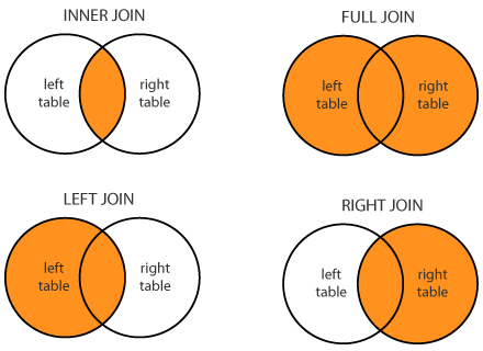
An inner_join puts together columns from both tables where there are matching rows. If there are records in either table where the IDs don’t match, they are dropped.
A left_join will keep ALL the rows of your first table, then bring over columns from the second table where the IDs match. If there isn’t a match in the second table, then new values will be blank in the new columns.
A right_join is the opposite of that: You keep ALL the rows of the second table, but bring over only matching rows from the first.
A full_join keeps all rows and columns from both tables, joining rows when they match.

Here are two common ways to think of this visually.

In the image below, The orange represents the data that remains after the join.

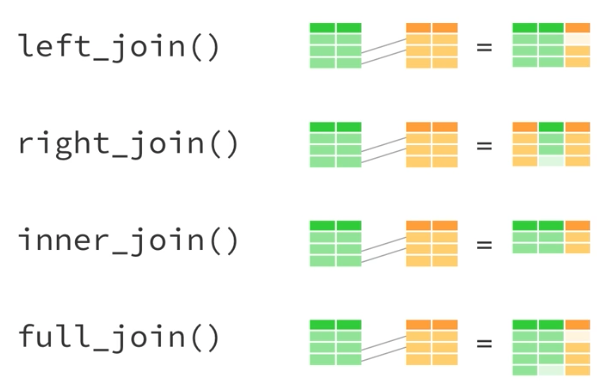
This next visual shows this as tables where only two rows “match” so you can see how non-matches are handled (the lighter color represents blank values). The functions listed there are the tidyverse versions of each join type.

10.6.1 Joining our reference table

In our case we will start with the dref data and then use an inner_join to add all the yearly data values. We’re doing it in this order so the dref values are listed first in our resulting table.

Start a new Markdown section and note we are joining the reference data
Add the chunk below and run it

1sped_joined <- dref |>
2  inner_join(dstud, by = "district")

sped_joined |> head()

1: We are creating a new bucket sped_joined to save our data. We start with dref so those fields will be listed first in our result.
2: We then pipe into inner_join() listing the dstud object, which will attach our dref data to our merged data when the ID matches in the district variable. The by = "district" argument ensures that we are matching based on the district column in both data sets.

We could’ve left out the by = argument and R would match columns of the same name, but it is best practice to specify your joining columns so it is clear what is happening. You wouldn’t want to be surprised to join by other columns of the same name. If you wanted to specify join columns of different names it would look like this:

# don't use this ... it is just an example 
df1 |> inner_join(df2, by = c("df1_id" = "df2_id"))

You should also glimpse() your new data so you can see all the columns have been added.

Add text that you are peeking at all the columns.
Add the code below and run it

sped_joined |> glimpse()

Rows: 13,087
Columns: 9
$ district <chr> "001902", "001902", "001902", "001902", "001902", "001902", "…
$ cntyname <chr> "ANDERSON", "ANDERSON", "ANDERSON", "ANDERSON", "ANDERSON", "…
$ distname <chr> "CAYUGA ISD", "CAYUGA ISD", "CAYUGA ISD", "CAYUGA ISD", "CAYU…
$ dflchart <chr> "N", "N", "N", "N", "N", "N", "N", "N", "N", "N", "N", "N", "…
$ dflalted <chr> "N", "N", "N", "N", "N", "N", "N", "N", "N", "N", "N", "N", "…
$ dpetallc <dbl> 595, 553, 577, 568, 576, 575, 564, 557, 535, 574, 593, 1236, …
$ dpetspec <dbl> 73, 76, 76, 78, 82, 83, 84, 82, 78, 84, 83, 113, 107, 126, 14…
$ dpetspep <dbl> 12.3, 13.7, 13.2, 13.7, 14.2, 14.4, 14.9, 14.7, 14.6, 14.6, 1…
$ year     <chr> "2013", "2014", "2015", "2016", "2017", "2018", "2019", "2020…

There are now 13087 rows in our joined data, fewer than what was in the original merged file because some districts (mostly charters) have closed and were not in our reference file. We are comparing only districts that have been open during this time period. For that matter, we don’t want charter or alternative education districts at all, so we’ll drop those next.

10.7 Some cleanup: filter and select

Filtering and selecting data is something we’ve done time and again, so you should be able to do this on your own.

You will next remove the charter and alternative education districts. This is a judgement call on our part to focus on just traditional public schools. We can always come back later and change if needed.

You’ll also remove and rename columns to make the more descriptive.

Start a new markdown section and note you are cleaning up your data.
Create an R chunk and start with the sped_joined and then do all these things …
Use filter() to keep rows where:
- the dflalted field is “N”
- AND the dflchart field is “N”
Use select() to:
- remove (or not include) the dflalted and dflchart columns. (You can only do this AFTER you filter with them!)
Use select() or rename() to rename the following columns:
- change dpetallc to all_count
- change dpetspec to sped_count
- change dpetspep to sped_percent
Make sure all your changes are saved into a new data frame called sped_cleaned.

I really, really suggest you don’t try to write that all at once. Build it one line at a time so you can see the result as you build your code.

Seriously, try on your own first

sped_cleaned <- sped_joined |> 
  filter(dflalted == "N" & dflchart == "N") |> 
  select(
    district,
    distname,
    cntyname,
    year,
    all_count = dpetallc,
    sped_count = dpetspec,
    sped_percent = dpetspep
  )

You should end up with 11225 rows and 7 variables.

10.8 Create an audit benchmark column

Part of this story is to note when a district is above the “8.5%” benchmark the TEA penalized them in their audit calculations. It would be useful to have a column that noted if a district was above or below that threshold so we could plot districts based on that flag. We’ll create this new column and introduce the logic of if_else().

OK, our data looks like this:

sped_cleaned |> head()

We want to add a column called audit_flag that says ABOVE if the sped_percent is above “8.5”, and says BELOW if it isn’t. This is a simple true/false condition that is perfect for the if_else() function.

Add a new Markdown section and note that you are adding an audit flag column
Create an r chunk that and run it and I’ll explain after.

1sped_flag <- sped_cleaned |>
2  mutate(audit_flag = if_else(
3    sped_percent > 8.5,
4    "ABOVE",
5    "BELOW"
  ))

# this pulls 10 random rows so I can check results
sped_flag |>
6  sample_n(10) |>
7  select(distname, sped_percent, audit_flag)

1: We’re making a new data frame called sped_flag and then starting with sped_cleaned.
2: We use mutate() to create a new column and we name it audit_flag. We set the value of audit_flag to be the result of an if_else() function.
3: The if_else function takes three arguments and the first is a condition test (sped_percent > 8.5 in our case). We are looking inside the sped_percent column to see if it is greater than “8.5”.
4: The second argument is what we want the result to be if the condition is true (the text “ABOVE” in our case.)
5: And the third argument is the result if the condition is NOT true (the text “BELOW” in our case).
6: Lastly we print out the new data sped_cleaned and pipe it into sample_n() which gives us a number of random rows from the data. I do this because the top of the data was all TRUE so I couldn’t see if the mutate worked properly or not. (Always check your calculations!!)
7: I’m using select() here to grab just the columns of interest for the check.

Be sure to look through the result to check the new audit_flag has values as you expect.

10.9 Export the data

This is something you’ve done a number of times as well, so I leave you to you:

Make a new section and note you are exporting the data
Export your sped_flag data using write_rds() and save it in your data-processed folder.

In the next chapter we’ll build an analysis notebook to find our answers!

10.10 New functions we used

list.files() makes a list of file names in a folder. You can use the pattern = argument to search for specific files to include based on a regular expression.
map() Loops through a vector or list and applies a function to each item. We used it with read_csv() to import multiple files and put them into a list.
list_rbind() is a function to combine elements into a data frame by row-binding them. In other words, it stacks them on top of each other into one thing.
set_names() provides a name to each element in a vector. We used it to add the “basename” of each file.
str_c() is used to combine text.
str_sub() allows us to extract part of a string based on it’s position.
We used inner_join() to add columns from one data frame to another one based on a common key in both objects.
if_else() provides specified results based on a true/false condition.

In later years we use Student Membership: Counts/Percents, a nuance added by the TEA in 2019-20 and outlined in the TAPR Glossary.↩︎
The name changes to “Student Enrollment by Instructional Programs” in later years.↩︎
The 2023 District Reference file from the TEA was missing some variables.↩︎